Stirling's Approximation, Paramagnetism, and Einstein Solids
Stirling's approximation
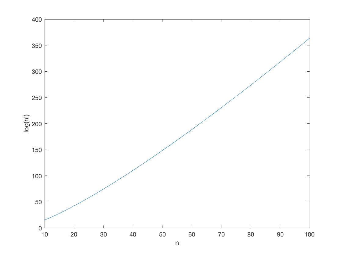
How large is \(n!\), and how accurate is Stirling's approximation? To refresh our memory about Matlab, and to get a feel for just how HUGE some of these numbers are, let's make a plot of \(\log(n!)\).
n = 100;
r = 10:n;
lognfac = log(factorial(r));
plot(r,lognfac);
xlabel('n'); ylabel('log(n!)');
How many digits are there in 100! ?
floor(log10(factorial(100)))+1
ans =

   158
158 digits! By contrast, \(10^{100}\) only has 100 digits. So 100! is much, much bigger than a googol. The total number of atoms in the whole universe is estimated to be \(10^{80}\) or there about. Thus 100! is roughly the square of the number of particles in universe!
Stirling's approximation is the following:
\(\log(n!) = n \log(n) - n + \frac{1}{2} \log(2\pi n) + O(1/n)\,.\)
Often only the first two terms are good enough for applications. Occasionally the third term is also relevant. How accurate is this? Let's plot the residual error
a1 = r.*log(r);
a2 = a1 - r;
a3 = a2 + .5*log(2*pi*r);

approx1 = abs( lognfac - a1 );
approx2 = abs( lognfac - a2 );
approx3 = abs( lognfac - a3 );

plot(r,approx1,r,approx2,r,approx3);
title('Absolute error for k terms in Stirling approximation');
xlabel('n'); ylabel('|log(n!) - a_n|');
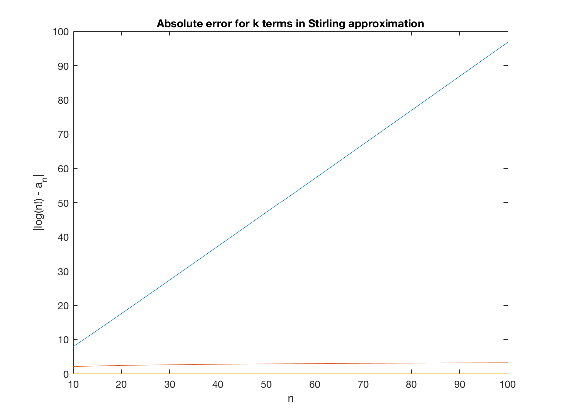
Looks like the first approximation is not so good. What is the percent error for each of these approximations?
relapprox1 = approx1./lognfac;
relapprox2 = approx2./lognfac;
relapprox3 = approx3./lognfac;

plot(r,relapprox1,r,relapprox2,r,relapprox3);
title('Relative error for k terms in Stirling approximation');
xlabel('n'); ylabel('|1 - a_k / log(n!)|');
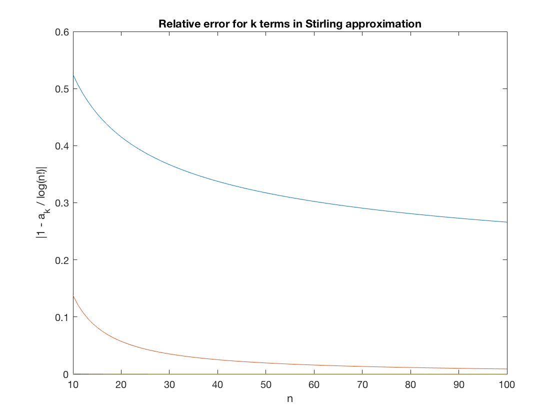
As you can see, the percent error is already quite small for the two-term approximation. By the third, it's totally negligable.
Flipping coins
Suppose we have a coin that lands heads with p=.5 (a fair coin), and we flip it 50 times.
n=50;
p=.5;
- How many possible outcomes are there?
- How many ways are there of getting 25 heads and 25 tails?
- What is the probability of getting exactly 25/25, in any order?
- What is the probability of getting 30/20, in any order? 40/10?
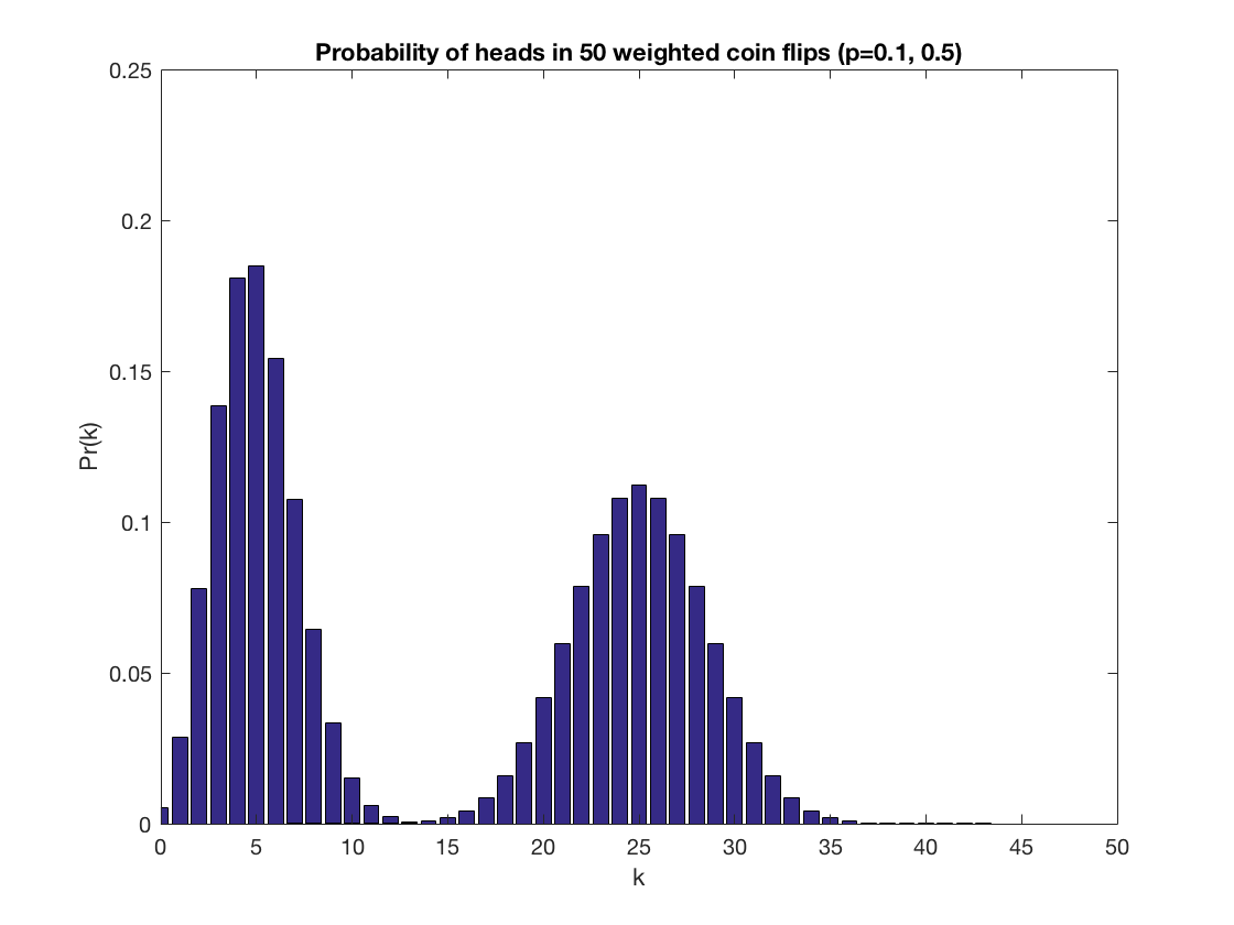
- Plot a graph of Pr(k) where k is the number of heads.
- Repeat that plot for several values of p.
k=25;
nchoosek(n,k) % number of ways to get k heads in n flips
ans*p^k*(1-p)^(n-k) % probability of k head in n flips

% Define a function for the probability of k heads
binom = @(n,k,p) nchoosek(n,k)*p^k*(1-p)^(n-k);

% Here is a combined plot for two values, p=0.1 and p=0.5.
for p=[.1,.5]
    b=zeros(n+1,1);
    for k = 0:50
        b(k+1) = binom(n,k,p);
    end
    figure(1)
    bar(0:50,b)
    hold on
end
title('Probability of heads in 50 weighted coin flips (p=0.1, 0.5)');
axis([0 50 0 0.25]);
xlabel('k'); ylabel('Pr(k)');
hold off
ans =

   1.2641e+14


ans =

    0.1123
Two-level Paramagnet
A paramagnet is a system which only has magnetization in the presence of an external magnetic field. This is in contrast with a ferromagnet which has strong interactions between the atoms (or molecules, etc.) that can cause it to retain a magnetization even in the presence of zero external field. A simple model for a paramagnet is a collection of \(n\) non-interacting particles with two energy levels each. We are going to consider just a single particle.
The energy levels of a paramagnet are described by the energy function
\(E_{\mu} = -\vec{\mu}\cdot \vec{B} = - \mu B \cos \theta\,.\)
The two-state paramagnet can only be either aligned or antialigned with the magnetic field, so the only allowed energy levels are \(\pm \mu B\). The aligned state has the lower (\(-\)) energy.
- What is the partition function for a single particle?
For a single particle, we just sum the exponentials of the energies:
\(Z = \e^{-\mu B/kT}+\e^{+\mu B/kT} = 2 \cosh(\mu B/kT)\,.\)
Now suppose that are collection of paramagnets are at \(T=300K\) (room temperature), so \(kT = .026\) eV. Suppose that \(\mu = 1\) eV/T.
- Compute the formula (as a function of the applied field \(\vec{B} = B\, \hat{z}\,\)) for the average energy.
- Compute the average magnetic moment
- Plot the both of these as a function of \(B\).
We can derive the first formula as follows:
\(\begin{aligned} \avg{E}\, & =(-\mu B) \e^{+\mu B/kT}/Z + (+\mu B) \e^{-\mu B/kT}/Z \\ & = (-\mu B) \frac{\e^{+\mu B/kT} - \e^{-\mu B/kT}}{2 \cosh(\mu B/kT)} \\ & = -\mu B \tanh(\mu B/kT)\,. \end{aligned}\)
The second formula is given by
\(\begin{aligned} \avg{\vec{\mu}\cdot \hat{z}}\, & = (+\mu) \e^{+\mu B/kT}/Z + (-\mu) \e^{-\mu B/kT}/Z \\ & = \mu \tanh(\mu B/kT)\,. \end{aligned}\)
We can plot these as follows:
kT = .026;
mu = 1;
B = -.1:.001:.1;
aveenergy = -mu*B.*tanh(mu*B/kT);
avemag = mu*tanh(mu*B/kT);
plot(B,avemag,B,aveenergy);
title('Average mu and E of 1eV paramagnet vs. B at 300 K');
xlabel('B (Tesla)'); legend('average \mu', 'average E');
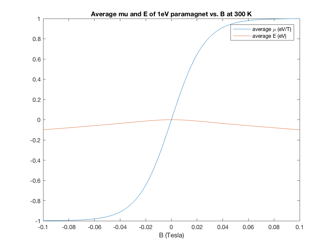
Note, \(.005 T\) is the strength of a typical refrigerator magnet, and \(0.15 T\) is the strength of a sunspot.
Einstein Solid
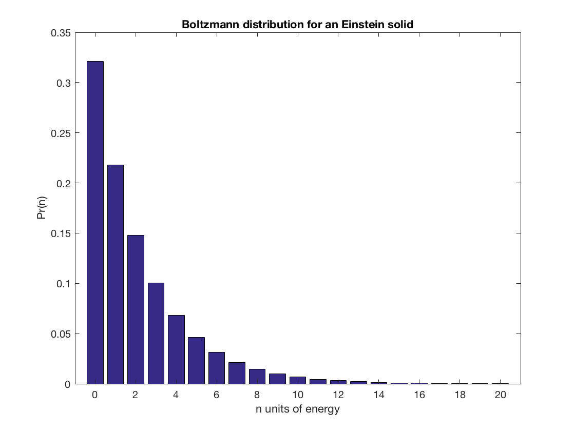
The monotonic decrease in Boltzmann probability weights does not contradict the fact that the mean energy (or whatever) could be peaked at high energy. To see this, let's consider the Einstein solid, a simple model of a solid material where we model each individual quantum system as a harmonic oscillator, and there are no interactions between the particles. Recall that for a one-dimensional quantum harmonic oscillator we can write these allowed energies as \(E_n = (n+\frac{1}{2})\hbar \omega\) for each nonnegative integer \(n\).
- What is the partition function of an Einstein solid with 1 eV of energy between energy levels? (Hint: this is a geometric series)
- Plot the Boltzmann distribution for several values of temperature.
- Plot the mean energy of the system at various temperatures.
k = 8.6e-5;
T = 30000; % Temperature in Kelvin
Z = 1/(2*sinh(1/(2*k*T))); % partition function
n=0:20; % energy level
p= exp(-(n+.5)/(k*T))/Z; % probability of being in level n
bar(n,p);
title('Boltzmann distribution for an Einstein solid');
axis([-1 21 0 .35]);
xlabel('n units of energy'); ylabel('Pr(n)');