Maxwell Speed Distribution
The Maxwell speed distribution for an ideal gas is
\(\displaystyle \mathcal{D}(v) \mathrm{d}v = \Bigl(\frac{m}{2\pi kT}\Bigr)^{3/2} 4\pi v^2 \e^{-mv^2/2kT}\mathrm{d}v\)
Let's define this as a function. We first notice that \(m\) and \(kT\) always occur together. So the only thing that matters for the physics is this ratio. Therefore, we define a new variable \(u = \sqrt{2kT/m}\) and express the speed distribution in terms of this quantity. You'll recall from class that \(u\) is just the most probable speed of a particle. To make things dimensionless, which is convenient for plotting purposes, we'll introduce \(x = v/u\). Then the probability density as a function of \(x\) is
\(\displaystyle \mathcal{D}(x)\mathrm{d}x = \frac{4}{\sqrt{\pi}} x^2 \e^{-x^2}\mathrm{d}x \quad , \quad u = \sqrt{\frac{2kT}{m}}\quad , \quad x=v/u\,.\)
The Maxwell speed distribution is a good approximation to the true speed distribution in an ideal gas when the mass \(m\) is small compared to \(kT\), i.e. when \(u\) is large.
maxwell = @(x) 4/sqrt(pi)* (x.^2).*exp(-x.^2);
Remember the interpretation of this formula: the probability of finding a particle with velocity in the range \(v\) and \(v+\dd v\) is given by
\(\mathcal{D}(v) \dd v\,.\)
As a sanity check, let's make sure this integrates to 1 when we integrate over all speeds.
integral(maxwell,0,Inf)
ans =

    1.0000
Here's a plot of the speed distribution in these dimensionless units.
ezplot(maxwell,[0,4])
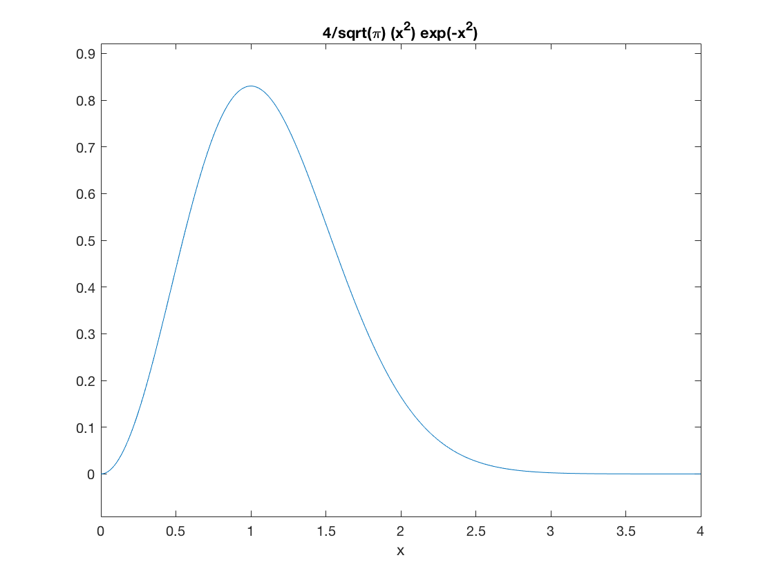
Again, we can visually check that the peak is at \(x=1\), meaning \(v=u\), as it should be.
Here is the first step in the derivation of the Maxwell speed distribution. We must compute the partition function. We can actually do this symbolically using the following commands.
% Define out variables
syms v m k T positive
% Define the integrand in the Partition function
% (degeneracy * Boltzmann factor)
z=4*pi*v^2*exp(-m*v^2/(2*k*T));
% Integrate to find the partition function
Z=int(z,v,0,inf);
% Output the dimensionful form
pretty(simplify(Z))
           3/2  3/2   3/2
2 sqrt(2) T    k    pi
-------------------------
            3/2
           m
Using the characteristic speed variable \(u\) introduced above, we can also simplify the result.
% Put in terms of the characteristic speed u
syms u positive
Z=subs(Z,T,m*u^2/(2*k));
% Output the new form
pretty(simplify(Z))
 3   3/2
u  pi
Of course, this integral can also be done with a change of variables and integration by parts, but it is nice to see that we can also do symbolic manipulations. The remainder of the derivation is left as an exercise.
Composition of the atmosphere
The Maxwell speed distribution can help us understand certain coarse features of our atmosphere.
The escape velocity of an object near the surface of the Earth is about 11 km/s. Particles traveling faster than this will leave the planet for good, assuming that they avoid any collisions on their way out.
In the thermosphere the temperature is actually quite high, more than 1000 K. (This is a bit misleading, because the atmosphere is so rarified at that altitude that a human would still freeze to death due to radiative heat loss before enough high-temperature gas particles collided with him or her.) At higher temperatures, energetic particles can reach higher speeds... but are these temperatures in the thermosphere enough for a particle to escape the clutches of Earth's gravitational field?
Let's see what will happen to a typical oxygen molecule in thermal equilibrium in the upper atmosphere. What is the probability that a randomly chosen molecule has a speed above the escape speed of 11 km/s?
kT = 1.38065e-23 * 1000; % Joules
mO2 = 2*16*1.66053892e-27; % atomic mass of oxygen molecule in kg
v_esc = 11000; % m/s, escape speed

u = sqrt(2*kT/mO2) % most probable speed in m/s

x_esc = v_esc/u % dimensionless escape speed;
u =

  720.8705


x_esc =

   15.2593
To escape, an oxygen molecule must be traveling more than 15 times the most probable speed, and 13.5 times greater than the average speed. Do we even need to compute the probability of escape? From the graph above, and the Gaussian decay of the Maxwell distribution, we can safely estimate that the fraction of escaping oxygen molecules is very close to zero.
integral(maxwell,x_esc,Inf)
ans =

  1.2963e-100
Yep. That's close to zero alright. Since there are fewer than \(10^{20}\) moles of oxygen molecules in the Earth's atmosphere, the probability that any of our oxygen is escaping due to temperature-induced speed fluctuations is totally negligable.
For hydrogen, it's another story. It is 16 times less massive than an oxygen molecule, so the most probable speed is 4 times greater.
mH2 = 2*1*1.66053892e-27; % atomic mass of hydrogen molecule in kg
v_esc = 11000; % m/s, escape speed

u = sqrt(2*kT/mH2) % most probable speed in m/s

x_esc = v_esc/u % dimensionless escape speed;
u =

   2.8835e+03


x_esc =

    3.8148
From the dimensionless escape speed, we can easily compute the probability that a hydrogen molecule has a large enough speed that it could escape.
integral(maxwell,x_esc,Inf)
ans =

   2.1276e-06
This is a small number, but nowhere near as small as for oxygen. It's clear that a substantial fraction of hydrogen molecules have left the Earth's atmosphere from this process.
The escape velocity of the moon is 2.4 km/s. What is the probability that an oxygen molecule will escape from the moon? (Assume a temperature of 1000 K still.)
v_esc_moon = 2400; % m/s, escape speed
u = sqrt(2*kT/mO2); % most probable speed in m/s
x_esc_moon = v_esc_moon/u; % dimensionless escape speed;

integral(maxwell,x_esc_moon,Inf)
ans =

   6.0169e-05
Now you should be able to explain: why does the moon have no atmosphere but the Earth does?
Blackbody radiation
Last class, you saw how the spectrum of electromagnetic radiation was distributed in thermal equilibrium. In particular, you considered the EM radiation inside a box with side length \(L\) and looked at the distribution of frequencies when at thermal equilibrium at a temperature \(T\). By assuming that the EM energy was quantized into units of \(hf\), you found that the partition function was
\(\displaystyle Z = \frac{1}{1-\e^{-\beta h f}}\,.\)
This implies that the average energy per unit is distributed according to
\(\displaystyle \bar{n}_{\text{Pl}} = \avg{n} = \frac{\avg{E}}{hf} = \frac{1}{\e^{h f/kT}-1}\,,\)
which is called the Planck distribution. This is a special case of the Bose-Einstein distribution when the chemical potential is set to zero, which can be regarded as a manifestation of the fact that photons can be either created or destroyed in any number whatsoever.
We can also ask about the total number of photons and the total energy inside the box. To do this, we need to count all of the modes and weigh them accordingly. As a warmup, consider the case of 1D. Here the wavelength of mode m inside the box is given by
\(\displaystyle \lambda_m = \frac{2L}{m}\,,\)
and the energy and momentum relations are simply
\(\displaystyle p_m = \frac{hm}{2L} \quad , \quad \eps = hf = \frac{hcm}{2L}\,.\)
In 3D, we use the generalization of this rule, and we find that the allowed energies are
\(\displaystyle \eps = \frac{hc}{2L}\sqrt{m_x^2+m_y^2+m_z^2} \,.\)
We can simplify this expression to make it look more like the previous one if we adopt the shorthand notation
\(\displaystyle \eps = \frac{hcm}{2L}\quad , \quad m = |\vec{m}|\,.\)
Now the total energy is given by a sum over all modes, namely
\(\displaystyle U = 2 \sum_{m_x,m_y,m_z=1}^\infty \eps \bar{n}_{\text{Pl}}(\eps) = 2 \sum_m \frac{hcm}{2L} \frac{1}{\e^{hcm/2LkT} -1}\,.\)
Here the factor of 2 comes from the sum over both polarization degrees of freedom per mode. As you saw with the density of states, we can turn this sum into an integral as follows,
\(\displaystyle U = \int_0^{\infty}\dd m \int_0^{\pi/2} \dd\theta \int_0^{\pi/2} \dd\phi(m^2 \sin \theta) \frac{hcm}{L}\frac{1}{\e^{hcm/2LkT} -1}\)
The integral runs only over the positive orthant of the sphere. If we change variables, we can do the simple angular integrals and rewrite the remaining radial integral in terms of the energy as follows
\(\displaystyle U = L^3 \int_0^\infty \dd\eps \frac{8\pi\eps^3/(hc)^3}{\e^{\eps/kT}-1}\,.\)
Dividing by the volume on each side, we can rewrite this as
\(\displaystyle \frac{U}{V} = \int_0^\infty u(\eps) \dd\eps \,,\)
where now the integrand is the energy density per unit photon energy. That is, \(u\) is the spectrum of the photons. It is worth writing it again separately:
\(\displaystyle u(\eps) =\frac{8\pi}{(hc)^3}\frac{\eps^3}{\e^{\eps/kT}-1}\,.\)
By changing variables, we can alternatively think of the spectrum as being a function either of the energy, the frequency, or the wavelength accordingly.
As usual, we can introduce a dimensionless variable \(x\) to help us study this quantity,
\(\displaystyle x = \frac{\eps}{kT}\,,\)
and now the energy density becomes
\(\displaystyle \frac{U}{V} = \frac{8\pi(kT)^4}{(hc)^3} \int_0^\infty\frac{x^3}{\e^{x}-1}\dd x = \frac{8\pi^5(kT)^4}{15(hc)^3}\,.\)
The final answer is in the last expression; the evaluation of the integral is not obvious, but is shown in Appendix B of the textbook. However, it is more important to notice two features about this expression. First, the integrand is still proportional to the Planck distribution, hence we can still interpret it as a probability density. That is, the probability of finding a mode with energy between \(x\) and \(x+\dd x\) is proportional to the density. Second, the energy density is proportional to the fourth power of \(kT\).
The high-frequency (short-wavelength) behavior of the spectrum is accurately captured by Wien's law, which predated Planck's derivation of the correct blackbody spectrum. It is just the lowest-order approximation to the blackbody spectrum. You can recover Wien's law in the case that the frequency is large compared to the temperature, in the sense that \(h \nu \gg kT\), and then the \(-1\) in the denominator of Planck's distribution becomes negligible. Similarly, the long wavelength, low energy behavior recovers the Rayleigh-Jeans law for the spectrum, in the opposite limit that \(h \nu \ll kT\). In this limit, one simply Taylor expands the exponential to derive the appropriate approximation.
Let's make a plot of the spectrum as a function of photon frequency (or energy), save for the overall factor of \(8\pi/(hc)^3\) which just serves to rescale the vertical axis.
u = @(x) x.^3./(exp(x)-1);
ezplot(u,0,12);
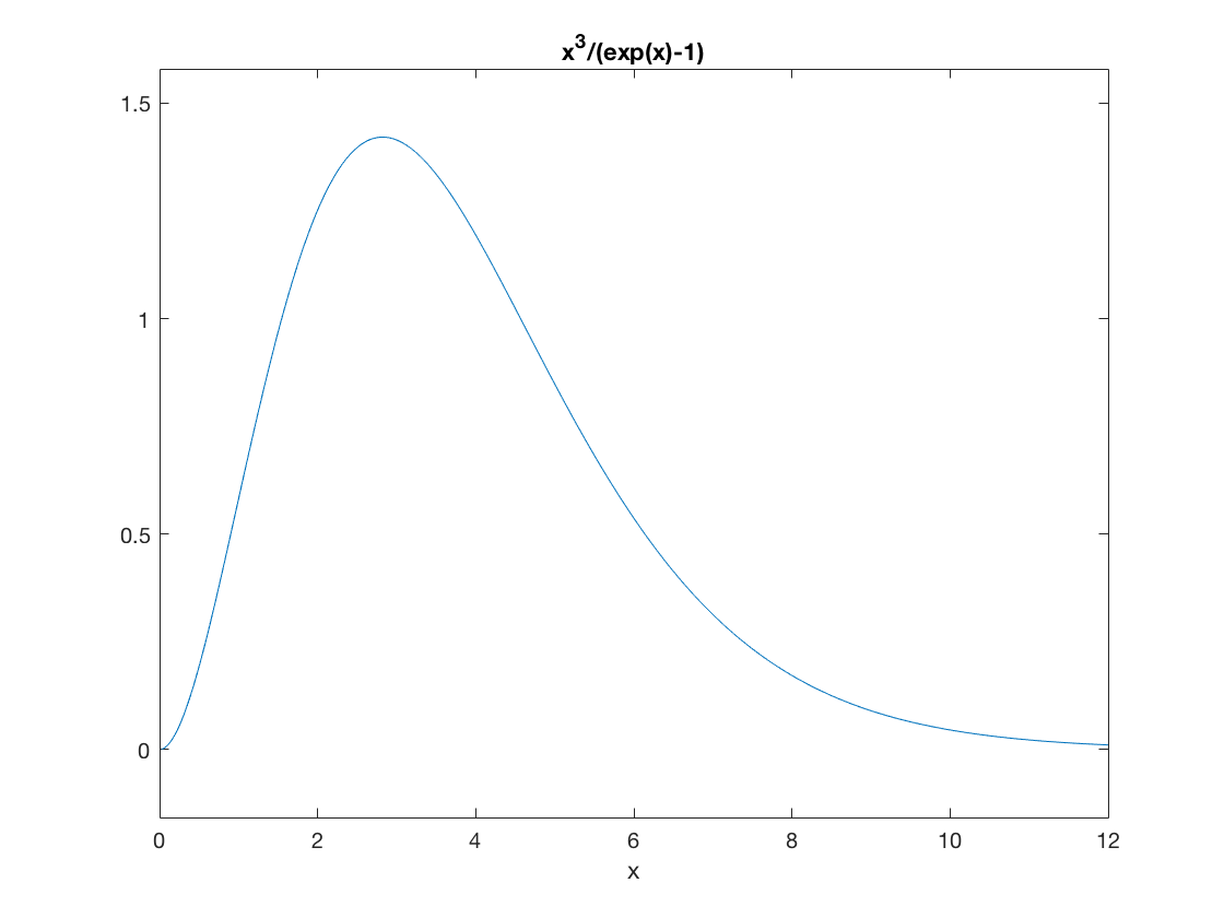
The peak value of this function occurs at \(x = 2.82\), or equivalently \(hf = 2.82 kT\). Thus, if you measure the relative intensity of radiation as a function of frequency for a blackbody and find the maximum, this will tell you the temperature.
If we add the dimensions back into the plot, then we can see the behavior of the blackbody spectrum as we change the temperature.
- Try to reproduce in Matlab the following plot of the Planck spectrum for various values of the temperature. Here they have divided out an overall constant factor, so don't worry about matching the vertical axis.
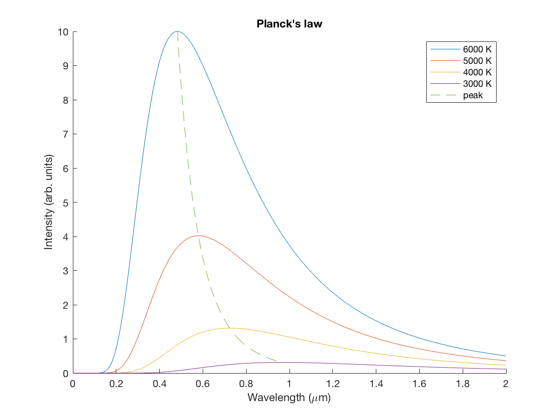
- Light sources are sometimes sold according to their "temperature", which does not correspond to the physical temperature of the source, but rather the temperature of the equivalently radiation blackbody. Which color light would be more appropriate for the lighting in a romantic Italian restaurant, 3000 K bulbs or 6000 K bulbs?
The sun is a blackbody and has a surface temperature of about 5800 K.
- At the sun's surface, how much energy is in the EM radiation within a cubic meter?
- What fraction of this energy is in the visible portion of the spectrum, with wavelengths between 400 nm and 700 nm?
C = 4.6356*1e-18; % k^4/(hc)^3 in units: J/(m^3 K^4)
T = 5800; % Kelvin
U = 8*pi^5*C*T^4/15 % energy in Joules
U =

    0.8562
Cosmic Background Radiation
Shortly after the Big Bang -- a mere 380,000 years later -- there was a sharp transition in the permeability of light through matter. This is known as the recombination epoch, and it corresponds to the time when the hot dense plasma in the early universe cooled sufficiently to allow the formation of neutral atoms. When this happened, it allowed for photon decoupling, meaning that photons were suddenly free to roam the universe without being repeatedly absorbed and re-emitted by the charged particles in the erstwhile plasma; that is, the mean free path of the photons suddenly increased dramatically. Since that time, the universe has continued to expand, and the the photon gas from the recombination epoch has continued to cool as well. (You can think of this as stretching the wavelengths of the photons; longer wavelengths = lower energies.)
The remnant of this still survives today in the form of the cosmic background radiation. As the universe has expanded about 1000-fold since the recombination epoch, the high-temperature gas of photons has cooled substantially in the more than 13 billion intervening years.
One of the triumphs of 20th century science was the discovery of this background radiation, and it is one of the major pieces of evidence in favor of the Big Bang model of cosmology, at least as important as Hubble's observations of the expanding universe. The original radiation was discovered by accident (!) in the 1960s, but today there are many precise measurements of the spectral density of these background photons.
One such measurement was done by the Cosmic Background Explorer (COBE) sattelite. The image below comes from the actual data from this sattelite.
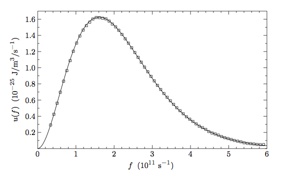
The continuous curve is a Planck distribution at a given temperature. By reading off the data from the graph:
- What temperature for the cosmic background radiation best explains the data? (Hint: use the peak value formula.)
- What is the typical wavelength of a cosmic background photon?