Debye vs. Einstein Solids

Previously, both in comp lab and in lecture, we studied the Einstein solid, a model of a solid that treats each constituent atom as an independent harmonic oscillator. We found that the heat capacity per particle in dimensionless units was given by \[\frac{C_V}{Nk}=\frac{3(\eps/kT)^2\e^{\eps/kT}}{(1-\e^{\eps/kT})^2}\,,\] where \(\eps = hf\) is the energy of the first excited state of the oscillator. Although the Einstein model gives qualitatively similar predictions to what is observed experimentally, the exponential drop in heat capacity for low temperatures does not agree quantitatively. The main problem is that each constituent particle in a solid does not oscillate independently from its neighbors.

The Debye model of a solid takes these collective oscillations into account, and more accurately reproduces the low-temperature behavior of solids with respect to their heat capacities. As we will see, one of the main ideas is to treat the occupation numbers in the oscillator modes with a Planck distribution, but with a high-frequency cutoff which is controlled by the lattice spacing between the particles. Although light waves can have arbitrarily short wavelengths, the shortest wavelength of sound waves in a solid is one half of the lattice spacing. Thus, the Debye model is a close solid-state analog of the blackbody radiation treatment of photons that we saw last class. All we are doing is treating the solid as a "phonon gas" in anology with a gas of photons, with a couple of important corrections, as we will see.

We begin with a solid cube of side length \(L\) and with \(N = L^3\) total constituent atoms or molecules. The wavelengths of standing waves along one axis of the box with mode number \(m\) are quantized according to \[\lambda_m = \frac{2L}{m}\,,\] where \(m\) is the mode number. The energy of one of these "phonons" is \[E_m\ =h f_m\,,\] where \(f_m\) is the frequency of the phonon. Treating these phonons as massless particles, we assume a dispersion relation that relates the energy (and hence the frequency) in inverse proportion to the wavelength. That is, we have an approximation given by \[E_m = h f_m=\frac{h c_{s}}{\lambda_m}=\frac{hc_s m}{2L}\,,\] where we define \(c_s\) to be the speed of sound inside the solid. The three-dimensional analog of this equation relates the length of the mode vector to the energy as follows, \[E_m = p_m c_s=\frac{hc_s}{2L}\sqrt{m_x^2+m_y^2+m_z^2} = \frac{hc_s}{2L}m\,,\] where \(p_m\) is the magnitude of the phonon momentum and \(m = \sqrt{\mathbf{m}\cdot\mathbf{m}}\) is the length of the mode vector \(\mathbf{m}\).

Note that the energy only depends on the length of the mode vector, not the direction. This is because we have assumed that the dispersion relation is isotropic, which is a natural assumption for a homogeneous medium, but will not always be true for real materials. For example, crystal structure might lead to varying speed of sound along different lattice directions. In fact, the speed of sound could in general depend on the length of the mode number as well. We will only consider the simplest case and avoid these difficulties.

As we did with blackbody radiation, we would like to derive expressions for the total energy and the spectrum. We will also derive the heat capacity.

Beginning with the total energy, we can compute this by simply summing over all of the modes times their average occupation number, \[U = 3 \sum_{\mathbf{m}} E_m\,\bar{n}(E_m) = 3 \sum_{m_x, m_y, m_z} E_m\,\bar{n}(E_m) \,,\] where \(\bar{n}(E_m)\) is the number of phonons with energy \(E_m\). Because phonons are bosons, the obey Bose–Einstein statistics, and the average occupation number is given by the familiar Bose–Einstein formula, \[\bar{n}(E) = \frac{1}{\e^{E/kT}-1}\,.\]

Compared to our derivation of Planck's law for blackbody radiation, we now come to still more differences. Phonons cannot have arbitrarily high frequencies, unlike photons, because the lattice spacing in the crystal sets a natural high-frequnecy cutoff. The following image is from Wikipedia, adapted from Schroeder:

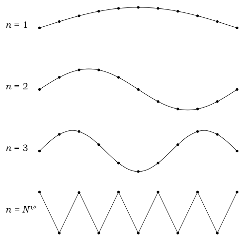
Here the illustration is in one dimension with mode number \(n\), but the key point is that after the mode number reaches \(L = N^{1/3}\) in one dimension, there are no higher frequency modes along that lattice direction. Thus, \(1\le m_x\le L\), and similarly for the other components of the mode vector. This sets the upper bound for the summation in the expression for the total energy.

Also, there is the issue of the factor of 3 appearing in front of \(U\). This factor comes in where only a 2 was present in our derivation of Planck's law. This is because there are three ways that a phonon can propagate: in addition to the transverse direction having (say) left and right circular polarization, the longitudinal mode can also contribute to the energy.

We now make another approximation, known as the Thomas–Fermi approximation, that the sum over the modes can be replaced by an integral, \[U = 3 \int_0^L\int_0^L\int_0^L E_m\,\bar{n}\bigl(E_m\bigr)\,\dd m_x\, \dd m_y\, \dd m_z\,.\] After substituting the definitions of the Bose-Einstein distribution and the energy, this becomes \[U = 3 \int_0^L\int_0^L\int_0^L \frac{hc_s m}{2L}\frac{1}{\e^{hc_s m/2L\,kT}-1}\,\dd m_x\, \dd m_y\, \dd m_z\,.\]

The integrand depends only on \(m\), not \(\mathbf{m}\), so we would like to transform again to radial coordinates. However, the region of integration is still that of a box. Debye's final insight into this problem was to just pretend that the boundary of the integration region was spherical anyway, since the modes at very high mode number do not contribute significantly to the integral. The new choice of spherical boundary radius \(R\) will be chosen to respect the total number of modes in the system, which is \(N = L^3\). This is illustrated in the following figure, adapted from Figure 7.27 in Schroeder.

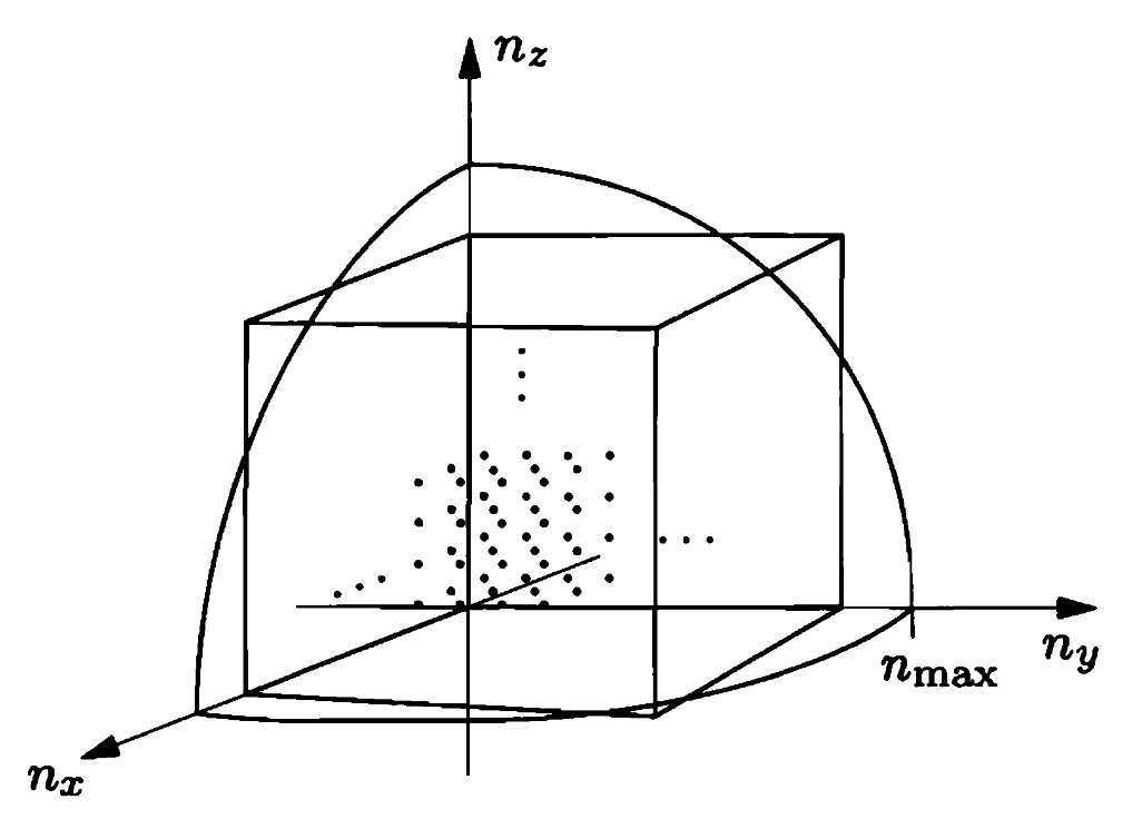
Transforming to spherical coordinates gives us the following integral for the total energy, \[U = 3 \int_0^{\pi/2}\int_0^{\pi/2}\int_0^R \frac{hc_s m}{2L}\frac{1}{\e^{hc_s m/2L\,kT}-1} m^2 \sin \theta \,\dd m\, \dd \theta\, \dd \phi\,,\] where the radius \(R\) will be chosen as follows. We wish to approximate a cube of side length \(L = N^{1/3}\) by an eighth of a sphere of radius \(R\), such that both shapes have the same volume. Therefore, \[N = L^3 = \frac{1}{8}\frac{4}{3}\pi R^3\,,\] or, solving for \(R\), we have \[R = \left(\frac{6N}{\pi}\right)^{1/3}\,.\] Solving the angular integrals and simplifying, we find \[U = {3\pi\over2}\int_0^R \,\frac{hc_sm}{2L}\frac{m^2}{\e^{hc_s m/2LkT}-1} \,\dd m\,.\] Now we can introduce a dimensionless change of variables by introducing \[x = \frac{hc_s m}{2LkT}\,.\] Then the integral becomes \[U = \frac{3\pi}{2} kT \left(\frac{2LkT}{hc_s}\right)^3\int_0^{hc_{\rm s}R/2LkT} \frac{x^3}{\e^x-1}\, \dd x\,.\]

At this point, we realize that there is a natural temperature scale that has emerged from our definition of the dimensionless parameter \(x\). When the mode number is maximized, we define a dimensionless variable \(x_\max\) which gives an upper bound on which frequecies of modes we will sum over, and we find that this bound corresponds to the Debye temperature \(T_D\), defined implicitly by \[x_\max = \frac{T_D}{T} = \frac{1}{T} \frac{h c_s}{2k} \biggl(\frac{6 N}{\pi V}\biggr)^{1/3} \,.\] This leads to a formula for the total average energy given by \[U=\frac{9NkT^4}{T_D^3}\int_0^{T_D/T} \frac{x^3}{\e^x-1}\dd x\,,\] and, after differentiating, the heat capacity is given by \[C_V= 9Nk\biggl(\frac{T}{T_D}\biggr)^3\int_0^{T_D/T}\frac{x^4\e^x}{(\e^x-1)^2}\dd x\,.\]

To accurately compare the Einstein and Debye solids, we have to make sure that we're summing over the same number of modes. Remember, Debye used a spherical integral to approximate the mode sum, whereas the Einstein model simply counts the number of modes in a cube. Therefore, we need a conversion factor \((\pi/6)^{1/3}\) to be able to compare the models. Let's plot the dimensionless heat capacities per particle predicted by both models for temperatures below the Debye temperature.

c = (pi/6)^(1/3);
CE = @(y) (c./y).^2.*exp(c./y)./(exp(c./y)-1).^2;
% This vectorizes the integral. 
CD = @(y) 3*y.^3.*integral( @(z) (1./y).*(z./y).^4.*exp(z./y)./(exp(z./y)-1).^2, ... 
        0, 1,'ArrayValued',1);

hold on;
ezplot(CD,[0,1]);
ezplot(CE,[0,1]);
hold off;
title('Comparison of Einstein and Debye heat capacities');
xlabel('$T/T_D$','interpreter','latex');
ylabel('$C_V/3Nk$','interpreter','latex');
legend('Debye','Einstein','Location','southeast');

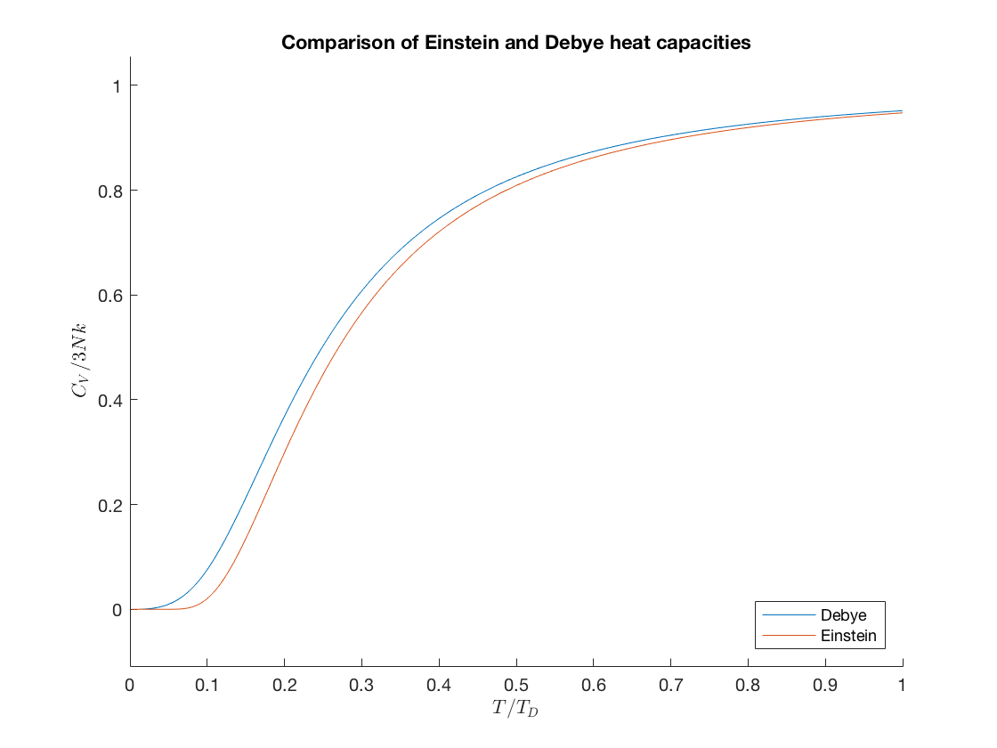
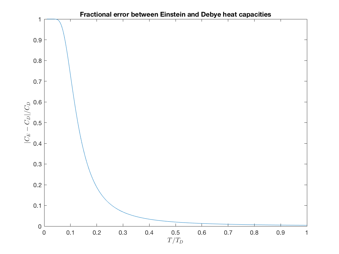
You might think, "What's the big deal? The Einstein model is close enough!" This is an artifact of the way we are plotting the data. In fact, the prediciton of the Einstein model is radically different from that of the Debye model. There are two ways to see this: looking at the percent error between the two models, and using a log plot to see the scaling behavior for low temperature.

r=.01:.001:1;
debye=CD(r); 
einstein=CE(r);
perror = abs(einstein-debye)./debye;
plot(r,perror)
title('Fractional error between Einstein and Debye heat capacities');
xlabel('$T/T_D$','interpreter','latex'); 
ylabel('$|C_E - C_D|/C_D$','interpreter','latex');

loglog(r,debye,r,einstein);
title('Log-Log plot of Einstein and Debye heat capacities');
xlabel('$T/T_D$','interpreter','latex'); 
ylabel('$C_V / 3NkT$','interpreter','latex');
legend('Debye','Einstein','Location','southeast');

As these two plots illustrate, below about half of the Debye temperature, the Einstein model really makes quite strikingly bad predictions (though it does still get the qualitative story correct).

Spin Waves and Ferromagnetism

A ferromagnet is a material that at small enough temperatures will spontaneously magnetize even in the absense of an external magnetic field. Iron is the classic example of a ferromagnet. Microscopically, the reason that some materials are ferromagnetic is that they have interactions between their constituent spins which energetically favor them to align along the same direction as their neighbors.

At zero temperature, the ferromagnet is perfectly polarized along a particular direction in space. (That direction is chosen spontaneously at random by quantum and thermal fluctuations as the magnet is cooled below a certain critical temperature.) The total magnetization for a system with \(N\) magnetic dipoles is then given by \(M = 2\mu_B N\), where \(\mu_B\) is the Bohr magneton.

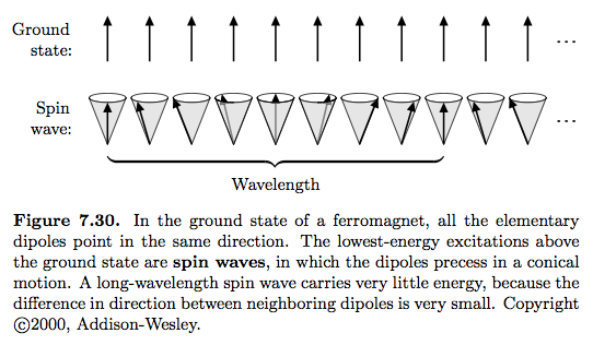
When \(T \gt 0\), there are excitations that take the form of spin waves. These are periodic precessions of the spins with a characteristic wavelength, as shown in the figure below taken from the text. Just like sound waves, these spin waves can only take energies in discrete quanta of energy, where the exact value is determined by the microscopic details of the ferromagnet such as the coupling strength and the lattice spacing. We can think of these discrete packets of energy as being particles (much like we did for phonons). These particles are called magnons.

One magnon changes the spin of the ferromagnet by \(h/2\pi\), hence the total magnetization decreases by about \(2 \mu_B\). In addition, each magnon carries with it an energy, and it has the same dispersion relation as a typical massive nonrelativistic particle, namely \[\eps = \frac{p^2}{2 m^*} \,,\] where \(m^*\) is an effective mass that again depends on the microscopic details of the material, and \[ p = \frac{hn}{2L} \] for a magnon with mode number \(n = (n_x,n_y,n_z)\) and \(L\) the size of the ferromagnet. This is in contrast to phonons, which behave in analogy with photons and have a linear energy-momentum dispersion relation. Magnons may also only be polarized in one possible direction (compared to photons which carry two polarizations or phonons which carry three).

The total number of magnons at a (low) temperature \(T\) should be given by the Planck distribution summed over all the magnon modes. We can do the same trick that we did for blackbody radiation and the Debye model and convert that sum over modes into an integral, and we get \[N_m = \frac{\pi}{2} \int_0^\infty \frac{n^2}{\e^{\eps/kT}-1}\dd n \,,\] where the upper limit is set to infinity because this picture only really holds at low temperatures. By changing variables to \(x = \eps/kT\), we can write this as \[N_m = 2\pi V \biggl(\frac{2m^*kT}{h^2}\biggr)^{3/2} \int_0^\infty\frac{\sqrt{x}}{\e^x-1} \dd x \,.\]

a = integral(@(x) x.^(1/2)./(exp(x)-1),0,Inf)

a =

    2.3152

If each magnon reduces the average magnetism by \(2\mu_B\), then the fractional decrease in magnetism at temperature \(T\) is simply \[ \frac{2 \mu_B N_m}{2 \mu_B N} = 2 \pi a \frac{V}{N} \biggl(\frac{2m^*kT}{h^2}\biggr)^{3/2} = \biggl(\frac{T}{T_0}\biggr)^{3/2}\,,\] where \[T_0 = \frac{h^2}{2 m^* k} \biggl(\frac{N}{2 \pi a V}\biggr)^{2/3}\,.\]

Magnons carry energy, hence they will contribute to the heat capacity of a material. If we follow the same mode-sum-to-integral method as before, we can compute the average total energy first to be \[U = 2\pi V k T \biggl(\frac{2m^*kT}{h^2}\biggr)^{3/2} \int_0^\infty\frac{x^{3/2}}{\e^x-1} \dd x \,.\]