Stirling's approximation and paramagnetism
Stirling's approximation
How large is \(n!\), and how accurate is Stirling's approximation? To refresh our memory about Matlab, and to get a feel for just how HUGE some of these numbers are, let's make a plot of \(\log(n!)\).
n = 100;
r = 10:n;
lognfac = log(factorial(r));
plot(r,lognfac);
xlabel('n'); ylabel('log(n!)');
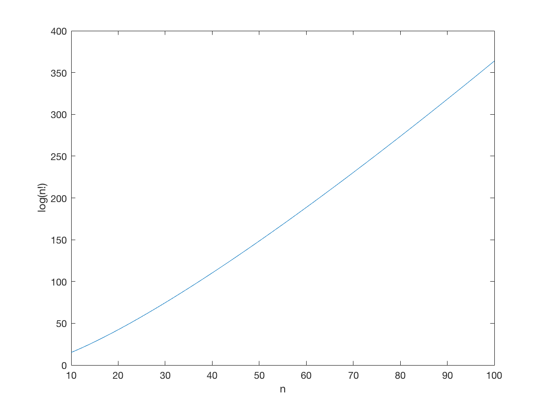
How many digits are there in 100! ?
floor(log10(factorial(100)))+1
ans =

158
158 digits! By contrast, \(10^{100}\) only has 100 digits. So 100! is much, much bigger than a googol. The total number of atoms in the whole universe is estimated to be \(10^{80}\) or there about. Thus 100! is roughly the square of the number of particles in universe!
Stirling's approximation is the following:
\(\log(n!) = n \log(n) - n + \frac{1}{2} \log(2\pi n) + O(1/n)\,.\)
Often only the first two terms are good enough for applications. Occasionally the third term is also relevant. How accurate is this? Let's plot the residual error
a1 = r.*log(r);
a2 = a1 - r;
a3 = a2 + .5*log(2*pi*r);

approx1 = abs( lognfac - a1 );
approx2 = abs( lognfac - a2 );
approx3 = abs( lognfac - a3 );

plot(r,approx1,r,approx2,r,approx3);
title('Absolute error for k terms in Stirling approximation');
xlabel('n'); ylabel('|log(n!) - a_n|');
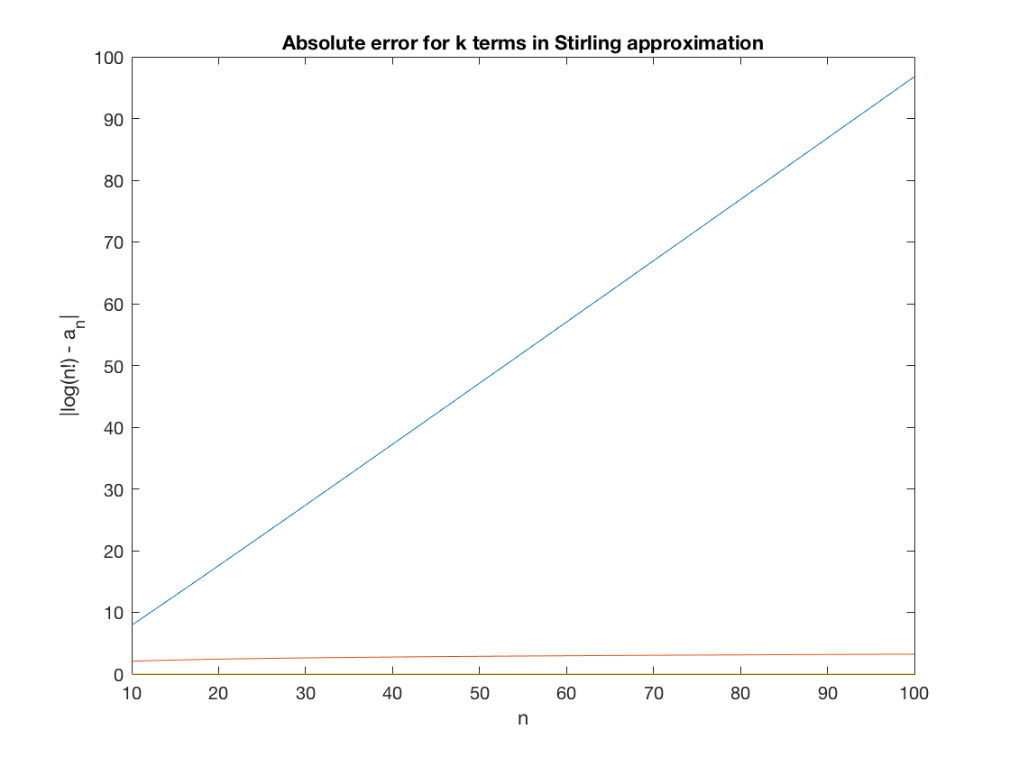
Looks like the first approximation is not so good. What is the percent error for each of these approximations?
relapprox1 = approx1./lognfac;
relapprox2 = approx2./lognfac;
relapprox3 = approx3./lognfac;

plot(r,relapprox1,r,relapprox2,r,relapprox3);
title('Relative error for k terms in Stirling approximation');
xlabel('n'); ylabel('|1 - a_k / log(n!)|');
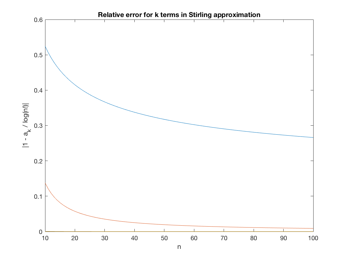
As you can see, the percent error is already quite small for the two-term approximation. By the third, it's totally negligable.
Flipping coins
Suppose we have a coin that lands heads with p=.5 (a fair coin), and we flip it 50 times.
n=50;
p=.5;
- How many possible outcomes are there?
- How many ways are there of getting 25 heads and 25 tails?
- What is the probability of getting exactly 25/25, in any order?
- What is the probability of getting 30/20, in any order? 40/10?
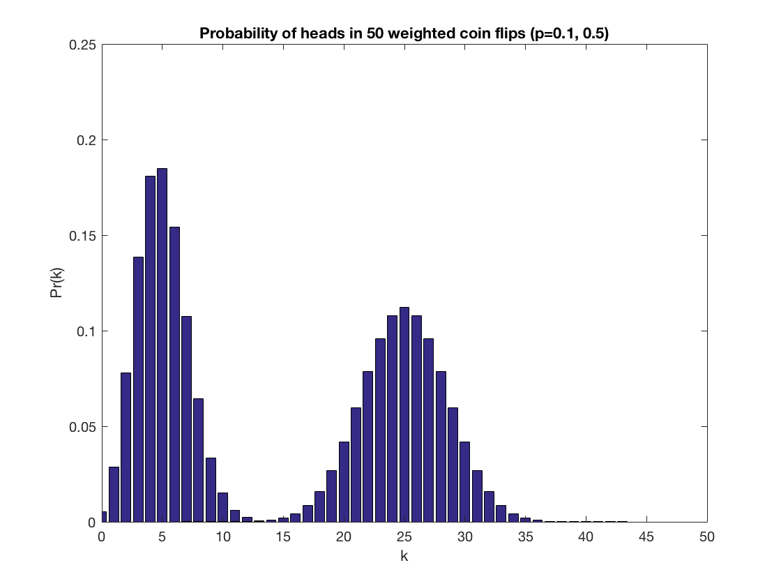
- Plot a graph of Pr(k) where k is the number of heads.
- Repeat that plot for several values of p.
k=25;
nchoosek(n,k) % number of ways to get k heads in n flips
ans*p^k*(1-p)^(n-k) % probability of k head in n flips

% Define a function for the probability of k heads
binom = @(n,k,p) nchoosek(n,k)*p^k*(1-p)^(n-k);

% Here is a combined plot for two values, p=0.1 and p=0.5.
for p=[.1,.5]
b=zeros(n+1,1);
for k = 0:50
    b(k+1) = binom(n,k,p);
end
figure(1)
bar(0:50,b)
hold on
end
title('Probability of heads in 50 weighted coin flips (p=0.1, 0.5)');
axis([0 50 0 0.25]);
xlabel('k'); ylabel('Pr(k)');
hold off
ans =

1.2641e+14


ans =

0.1123
Two-level Paramagnet
A paramagnet is a system which only has magnetization in the presence of an external magnetic field. This is in contrast with a ferromagnet which has strong interactions between the atoms (or molecules, etc.) that can cause it to retain a magnetization even in the presence of zero external field. A simple model for a paramagnet is a collection of \(n\) non-interacting particles with two energy levels each. We are going to consider just a single particle.
The energy levels of a paramagnet are described by the energy function
\(E_{\mu} = -\vec{\mu}\cdot \vec{B} = - \mu B \cos \theta\,.\)
The two-state paramagnet can only be either aligned or antialigned with the magnetic field, so the only allowed energy levels are \(\pm \mu B\). The aligned state has the lower (\(-\)) energy.
- What is the partition function for a single particle?
For a single particle, we just sum the exponentials of the energies:
\(Z = \e^{-\mu B/kT}+\e^{+\mu B/kT} = 2 \cosh(\mu B/kT)\,.\)
Now suppose that our collection of paramagnets is at \(T=300K\) (room temperature), so \(kT = .026\) eV. Suppose that \(\mu = 1\) eV/T.
- Compute the formula (as a function of the applied field \(\vec{B} = B\, \hat{z}\,\)) for the average energy.
- Compute the average magnetic moment
- Plot the both of these as a function of \(B\).
We can derive the first formula as follows:
\(\begin{aligned} \avg{E}\, & =(-\mu B) \e^{+\mu B/kT}/Z + (+\mu B) \e^{-\mu B/kT}/Z \\ & = (-\mu B) \frac{\e^{+\mu B/kT} - \e^{-\mu B/kT}}{2 \cosh(\mu B/kT)} \\ & = -\mu B \tanh(\mu B/kT)\,. \end{aligned}\)
The second formula is given by
\(\begin{aligned} \avg{\vec{\mu}\cdot \hat{z}}\, & = (+\mu) \e^{+\mu B/kT}/Z + (-\mu) \e^{-\mu B/kT}/Z \\ & = \mu \tanh(\mu B/kT)\,. \end{aligned}\)
We can plot these as follows:
kT = .026;
mu = 1;
B = -.1:.001:.1;
aveenergy = -mu*B.*tanh(mu*B/kT);
avemag = mu*tanh(mu*B/kT);
plot(B,avemag,B,aveenergy);
title('Average mu and E of 1eV paramagnet vs. B at 300 K');
xlabel('B (Tesla)'); legend('average \mu (eV/T)', 'average E (eV)');
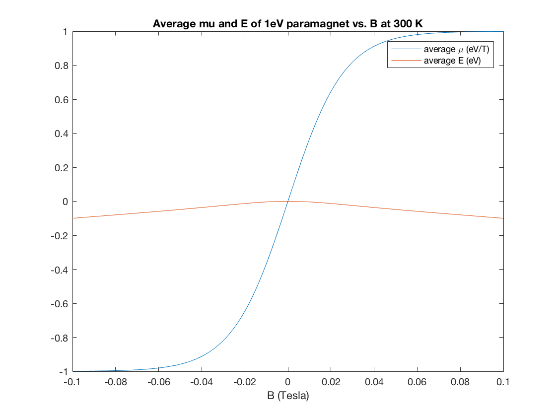
Note, \(.005 T\) is the strength of a typical refrigerator magnet, and \(0.15 T\) is the strength of a sunspot.