Paramagnetism
As we saw in the last lab and in class, a two-state paramagnet is a simple system where we can explore the Boltzmann factor and the associated physics. Let's review where we left off last time.
Suppose as before that each energy level has energy \(\pm \mu B\). Then the partition function for a single particle is just the sum of the exponentials of the energies divided by \(kT\):
\(Z=\e^{-\mu B/kT}+\e^{+\mu B/kT} = 2\cosh(\mu B/kT)\)
The probability of each configuration is then given by
\(\displaystyle \P_\uparrow = \frac{\e^{+\mu B/kT}}{Z} \quad , \quad \P_\downarrow = \frac{\e^{-\mu B/kT}}{Z}\)
The average energy is
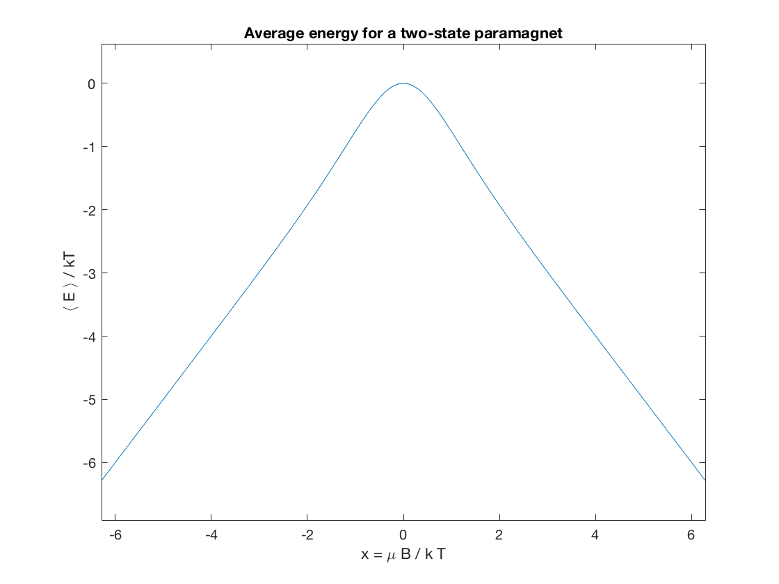
\(\avg{E} = -\mu B \tanh(\mu B/kT)\)
And the average magnetic moment along the \(\hat{z}\) axis is
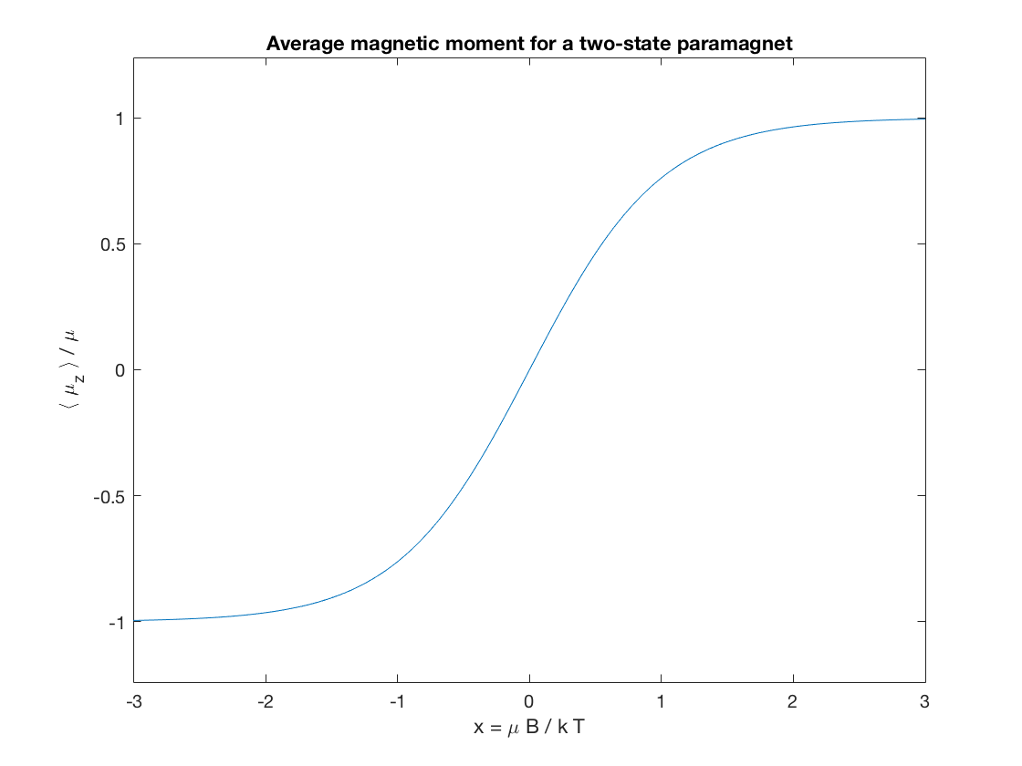
\(\avg{\vec{\mu}\cdot\hat{z}} = \mu \tanh(\mu B/kT)\)
Last time we plotted these with respect to certain given numbers for the temperature and the magnetic moment. This time we will use a powerful trick to help understand the behavior of functions which is obvious once you see it, but nevertheless can require some thought to apply in any given circumstance. The idea is that we should only ever plot quantities that are dimensionless quantities. This is because the units that we choose to use are arbitrary, and so our plots should be essentially independent of these arbitrary choices. Moreover, every problem in physics has one or more natural scales at which the physics is interesting.
As an example, notice how for thermal physics, \(kT\) is a natural unit of energy in every problem. There is a high-temperature limit, and a low-temperature limit, and the energy scales which determine which limit one is in are always relative to \(kT\).
With this insight in hand, let's replot the average energy and average magnetic moment from last time. It will be convenient to define the dimensionless parameter
\(\displaystyle x = \frac{\mu B}{kT}\,.\)
Our plots will now reflect this new dimensionless character by plotting the average energy in units of \(kT\).
aveE = @(x) -x.*tanh(x);
ezplot(aveE);
title('Average energy for a two-state paramagnet');
xlabel('x = \mu B / k T'); ylabel('\langle E \rangle / kT');
aveMu = @(x) tanh(x);
ezplot(aveMu);
title('Average magnetic moment for a two-state paramagnet');
xlabel('x = \mu B / k T'); ylabel('\langle \mu_z \rangle / \mu');
Fluctuations
Let's continue our investigation of paramagnetism by looking at the fluctuations of these quantities. One common measure of fluctuation is the standard deviation. For a given physical quantity \(X\), the standard deviation of \(X\) is determined by the formula
\(\sigma_X = \sqrt{\avg{X^2} - \avg{X}^2}\)
Thus, we need to know the average of the square of \(X\) in addition to knowing the average value of \(X\).
Let's compute the standard deviation in the energy.
\(\avg{E^2} = (-\mu B)^2 \P_\uparrow + (+\mu B)^2 \P_\downarrow = (\mu B)^2\,.\)
\(\avg{E}^2 = (\mu B)^2 \tanh^2(\mu B/kT)\)
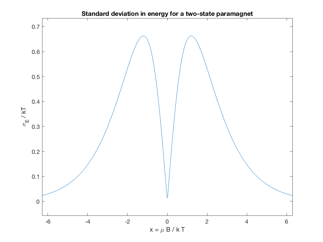
\( \sigma_E = \sqrt{\avg{E^2}-\avg{E}^2} = |\mu B|\sqrt{1-\tanh^2(\mu B/kT)} = |\mu B \,\mathrm{sech}(\mu B/kT)|\,.\)
Plotting this in terms of our dimensionless variable \(x\), we find
stdevE = @(x) abs(x.*sech(x));
ezplot(stdevE);
title('Standard deviation in energy for a two-state paramagnet');
xlabel('x = \mu B / k T'); ylabel('\sigma_E / kT');
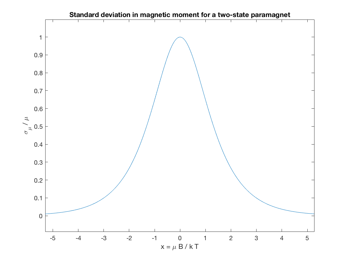
- Exercise: Reproduce the following plot for the standard deviation in the magnetic moment.
Derivatives of the Partition function
There is another important way to compute averages using the partition function. In fact, this way is rather remarkable in that you never need to explicitly compute the probabilities for the individual energies.
Recalling that \(\beta = 1/kT\), the two most important formulas are the following:
\(\displaystyle \avg{E} = \frac{-1}{Z}\frac{\partial Z}{\partial \beta} = -\frac{\partial \ln Z}{\partial \beta}\,,\)
\(\displaystyle \avg{E^2} = \frac{1}{Z}\frac{\partial^2 Z}{\partial \beta^2} \,.\)
- Exercise: using the command diff, use the derivative formulas above and redo the plots for for \(E\) and \(E^2\) above. Make sure that your plots are dimensionless.
Hint: we need to use the chain rule to get the correct answer. Since we have defined \(Z\) as a function of the dimensionless quantity \(x\) rather than \(\beta\), we have to use the following formula:
\(\displaystyle \frac{\partial Z}{\partial \beta} = \frac{\partial Z}{\partial x} \frac{\partial x}{\partial \beta}\,.\)
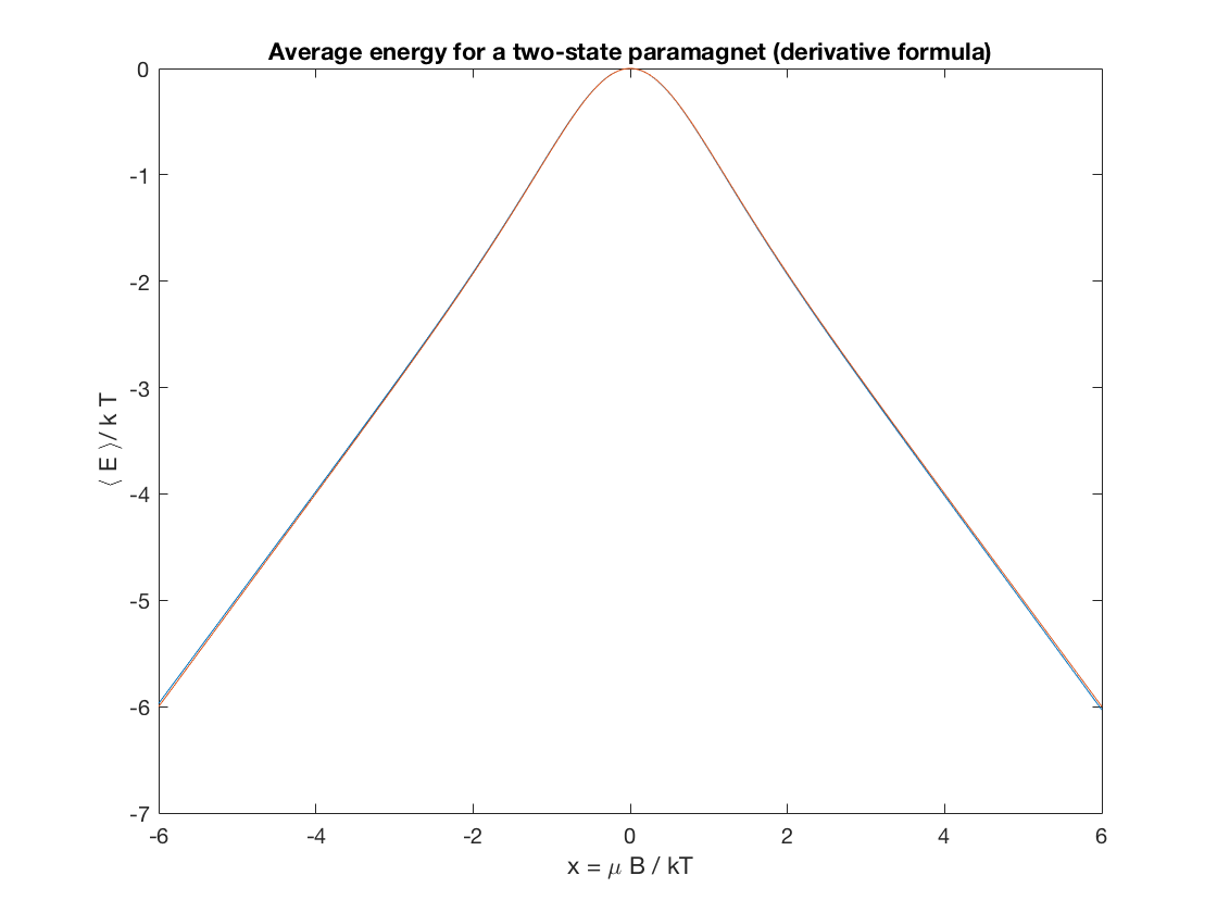
dx = .01; % choose a small interval
x = -6:dx:6;
x1 = -6:dx:(6+dx); % pad with an extra element so that diff works
Z = @(x) 2*cosh(x);

% Using the chain rule, we find the dimensionless average energy:
avgE = -1./Z(x).*(diff(Z(x1))/dx.*x);

% For comparision, here is the exact answer:
exactE = @(x) -x.*tanh(x);

plot(x,avgE,x,exactE(x));
title('Average energy for a two-state paramagnet (derivative formula)')
xlabel('x = \mu B / kT'); ylabel('\langle E \rangle/ k T');
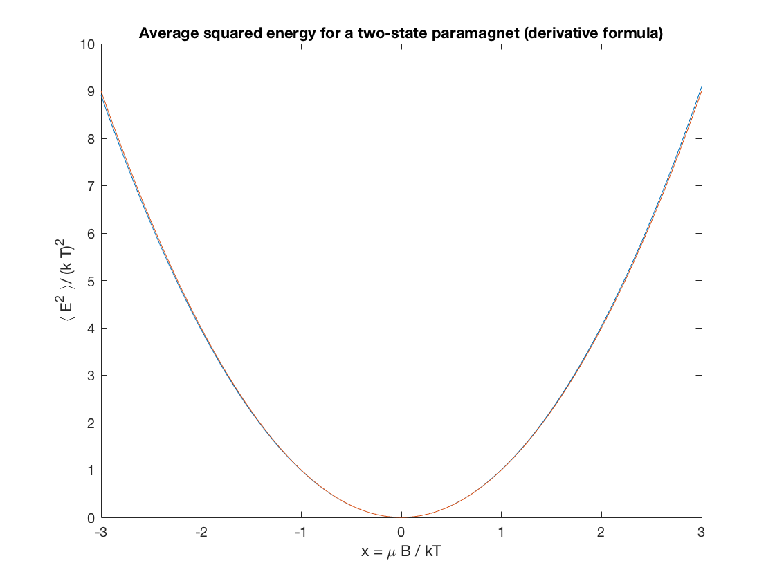
dx = .01;
x = -3:dx:3;
x2 = -3:dx:(3+2*dx); % pad with 2*dx for a second derivative

% Using the chain rule, we find the dimensionless quantity:
avgE2 = 1./Z(x).*(diff(Z(x2),2)/(dx^2).*x.*x) ;

% Here is the exact answer for comparision:
exactE2 = @(x) x.^2;

plot(x,avgE2,x,exactE2(x));
title('Average squared energy for a two-state paramagnet (derivative formula)')
xlabel('x = \mu B / kT'); ylabel('\langle E^2 \rangle/ (k T)^2');
- Exercise: Plot the absolute and relative error for the numerical approximations above.
Note that the numerical derivative is a bit sensitive to errors because of the finite size of dr. If you make dr a bit bigger, you can start to see the limitations of this approach. When working with noisy data in real life, it can be challenging to perform multiple numerical derivatives because of this instability. Therefore, we will mostly try to avoid using these derivative formulas in the comp lab. The derivative is still extremely useful for finding analytic expressions, however.