Einstein solid

The Einstein model of a solid is a very simple model which treats the system as a collection of noninteracting harmonic oscillators. Historically, this model was important because it was the first to give an explanation of the heat capacity of solids at low temperatures. Although the Debye model gives more accurate predictions, the Einstein model was the first to reproduce roughly the correct behavior. Because the model invoked quantum mechanics (specifically, quantized energy levels), it formed one of the key pieces of early evidence in favor of the quantization hypothesis.

In the full Einstein solid, we would consider a three-dimensional system with \(N\) particles. We will consider a simpler case with just a single one-dimensional quantum harmonic oscillator as the only particle. The quantum harmonic oscillator has energy levels given by

\(E_n = \bigl(n+\frac{1}{2}\bigr) \hbar \omega \,.\)

The partition function is given by

\(\displaystyle Z = \sum_{n=0}^\infty \e^{-\beta E_n} = \e^{-x/2} \sum_{n=0}^\infty \e^{-nx}\,\)

where, as usual, we introduce a dimensionless parameter \(x\) which here is given by

\(\displaystyle x=\frac{\hbar \omega}{kT}\,.\)

Because this sum is a geometric series, we can compute an exact expression for the partition function, namely

\(\displaystyle Z = \frac{1}{2 \sinh(x/2)}\,.\)

When an Einstein solid is in thermal equilibrium, the Boltzmann factor tells us the probability that there are exactly \(n\) excitations in a given oscillator. That is, we have

\(\displaystyle \begin{aligned} \P_n\, & = \frac{\e^{-\beta E_n}}{Z}\\ & = 2 \sinh(x/2) \e^{-x (n+1/2)}\\ & = (1-\e^{-x}) \e^{-xn}\,. \end{aligned}\)

Because there are an infinite number of energy levels in our system, we need to understand how to do a sensible calculation on a computer with only a finite number of energy levels. Of course, in this simple example there are exact expressions available, but doing things numerically will help us build intuition for the less simple cases.

Therefore, let us compute the following quantities in dimensionless units using the summation formulas above. Before computing them, think about how many terms you need to keep in the summation to get good agreement with the exact expressions given below.

The exact expressions are:

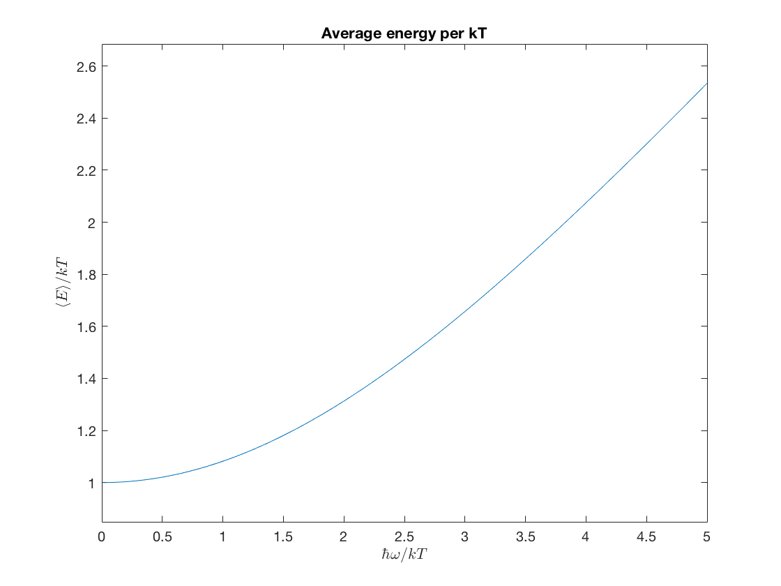
\(\displaystyle \frac{\avg{E}}{kT} = \frac{x}{2}\coth\frac{x}{2}\,,\)

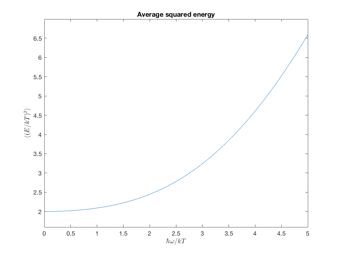
\(\displaystyle \frac{\avg{E^2}}{(kT)^2} = \frac{x^2}{4}\frac{\cosh(x)+3}{\cosh(x)-1}\,,\)

\(\displaystyle \frac{C}{k} = \frac{\sigma_E^2}{(kT)^2} = \bigl[2y \sinh(1/2y)\bigr]^{-2}\,,\)

where

\(\displaystyle y = \frac{1}{x} = \frac{kT}{\hbar \omega}\,.\)

Here are the exact plots for comparison:

aveE = @(x) .5*x.*coth(x./2);
ezplot(aveE,[0,5]);
% This fancy labeling uses LaTeX to make it look nice. 
xlabel('$\hbar\omega/kT$','interpreter','latex'); 
ylabel('$\langle E \rangle/kT$','interpreter','latex');
title('Average energy per kT');

aveEsq = @(x) .25*x.^2.*(cosh(x)+3)./(cosh(x)-1);
ezplot(aveEsq,[0,5]);
xlabel('$\hbar\omega/kT$','interpreter','latex'); 
ylabel('$\langle (E /kT)^2 \rangle$','interpreter','latex');
title('Average squared energy')

heatC = @(y) (2*y.*sinh(.5./y)).^(-2);
ezplot(heatC,[0,5,0,1]);
xlabel('$kT/\hbar\omega$','interpreter','latex');
ylabel('$C/k$','interpreter','latex');
title('Heat capacity');

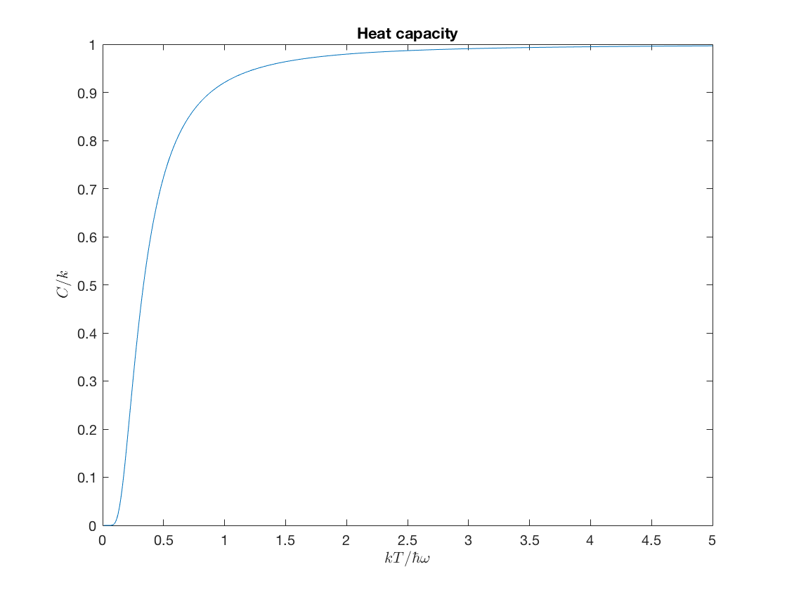
This last graph is very famous, because it showed how the quantization hypothesis could reproduce the decrease in specific heat at low temperatures that had been experimentally observed.

Anharmonic oscillators

In the Einstein solid, each particle is a perfect harmonic oscillator with equally spaced energy levels. In more realistic circumstances, the harmonic oscillator approximation breaks down for large \(n\), when the energy of the oscillator is comparable to certain other energy scales in the problem. For example in a diatomic molecule like \(\mathrm{H}_2\), which we'll study in more detail next class, there is a characteristic energy associated with the covalent bond between the hydrogen atoms. When \(kT\) is large compared to this energy scale, then thermal fluctuations can cause the molecule to disassociate.

One simple way to model this is to add a small amount of anharmonicity to the energy spectrum of the system. Let's consider a system whose energy levels are given by

\(E_n = E_0\bigl(n-\frac{\eps}{2}n^2\bigr)\)

for small values of \(n\), and where \(\eps\) is a small parameter of the model. (The factor of 2 is for convenience.) When \(\eps\) is zero, we recover the equal energy spacing of a harmonic oscillator, but when \(\eps\) is a small positive number there are corrections. When \(n\) becomes large, the energies become negative, so we know this formula can't hold for all \(n\).

Now let's choose a small value of \(\eps\); since it is dimensionless, we can choose .05, say, without reference to any units in the problem.

eps = .05;
En = @(n) n-.5*eps* n.^2;
ens = En(1:20);

Here we compute the partition function, the average energy, and the heat capacity (in dimensionless units).

Z = @(b) sum(exp(-ens'*b));
% This divides the matrix by the vector column-by-column
p = @(b) exp(-ens'*b)./Z(b);

% Now these average quantities can be done as dot products
aveE = @(b) ens*p(b);
aveEsq = @(b) (ens.^2)*p(b);

Lastly, plot the heat capacity versus Temperature

heatC = @(b) b.^2.*(aveEsq(b)-aveE(b).^2);
ezplot(@(z) heatC(1./z'),[0,4]);
title('Heat capacity vs. temp');
xlabel('$kT/E_0$','interpreter','latex'); 
ylabel('$C/k$','interpreter','latex');

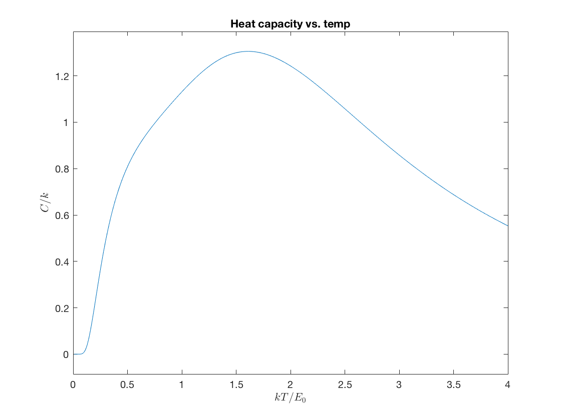
How do these results change when you keep fewer energy levels? Can you give an interpretation for why the heat capacity should decrease at larger temperatures for this system?

Thinking About Numerical Approximation Error

The key insight is that when \(n\) is large compared to the dimensionless quantity \(x\), then the probability decreases very quickly, and the average values do too. Therefore, if we want to plot a range of values up to some maximum value x, then we need \(n \gg x\).

Let us return to the Einstein solid. For comparison, let's first define the exact answers that we get from summing a geometric series. These answers are in units of \(kT\). (You could also compute the average energy in units of \(\hbar \omega\)... how would the answers change in that case?)

aveE_exact = @(x) .5*x.*coth(x./2);
aveEsq_exact = @(x) .25*x.^2.*(cosh(x)+3)./(cosh(x)-1);
heatCtemp_exact = @(y) (2*y.*sinh(.5./y)).^(-2);

Next let's define approximate versions where we only sum over the first n energy levels to get an approximate answer.

% sum only the first n energy levels in the partition function
Z_approx = @(x,n) sum(exp(-( (0:n)+.5 )'*x));

% average only the first n energy levels for the average energy
aveE_approx = @(x,n) x.*( ((0:n)+1/2 )*exp(-( (0:n)+.5 )'*x) )./Z_approx(x,n);

% average squared energy and heat capacity (versus y = 1/x)
aveEsq_approx = @(x,n) x.^2.*( (((0:n)+1/2).^2 )*exp(-( (0:n)+.5 )'*x) )./Z_approx(x,n);
heatC_approx = @(x,n) (aveEsq_approx(x,n) - aveE_approx(x,n).^2);

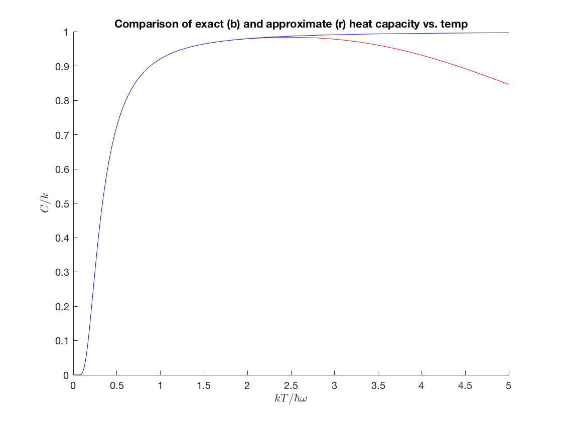
Now let's see what the approximate heat capacity looks like versus temperature. You should play around and see how large \(n\) has to be before we get good agreement at a given (dimensionless) temperature.

n = 25;
a = ezplot(@(x) heatC_approx(1./x',n),[0,5,0,1.02]);
hold on;
b = ezplot(heatCtemp_exact,[0,5,0,1]);
set(a, 'Color', 'r');
set(b, 'Color', 'b');
hold off;
title('Comparison of exact (b) and approximate (r) heat capacity vs. temp');
xlabel('$kT/\hbar\omega$','interpreter','latex');
ylabel('$C/k$','interpreter','latex');