Rotation of Diatomic Molecules
We will begin by considering heteronuclear diatomic molecules, i.e. those which have two different atomic species.
The classical expression for the energy of rotation is given by
\(\displaystyle E = \frac{L^2}{2I}\,,\)
where \(L\) is the angular momentum and \(I\) is the moment of inertia, which is given in terms of the average internuclear spacing \(r\) and the masses of the constituent nuclei by
\(\displaystyle I = \frac{m_1m_2}{m_1+m_2}r^2\,.\)
For a quantum mechanical system, the allowed values of the angular momentum are quantized, and the operator \(L^2\) can only take the values
\(j(j+1)\hbar^2\ , \quad j=0,1,2,\ldots\)
Moreover, the \(j\)th energy level is (\(2j+1\))-fold degenerate. Thus, the energy level structure is given by the following figure (Fig. 6.6 from your book)
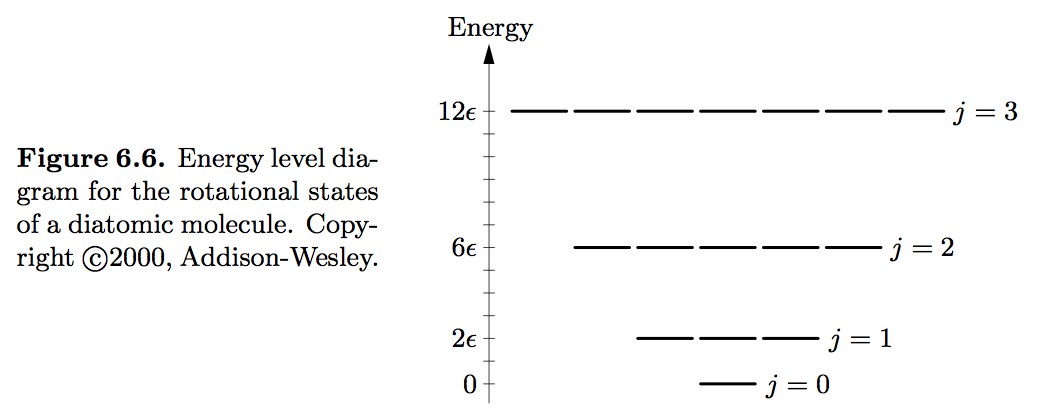
Let's now define the characteristic energy of rotation for a given molecule by
\(\displaystyle \eps = \frac{\hbar^2}{2I}\,,\)
which is just half the energy between the ground and first excited state. Then the energy levels of the molecule are given by
\(E_j = j(j+1) \eps\,.\)
A dimensionless quantity that captures how large the thermal energy is compared to this characteristic energy is
\(\displaystyle x=\frac{kT}{\eps}\,.\)
By now we know that the first thing to do is compute the partition function, so let's do that, keeping in mind that the energies for this system are degenerate.
\(\displaystyle Z = \sum_{j=0}^\infty (2j+1) \e^{-j(j+1)\eps/kT}\)
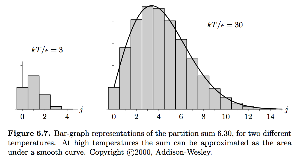
This sum cannot be evaluated exactly, but we can extract the relevant physics by considering various limits. Most often, we are interested in the regime where the sum can be replaced with an integral. This is because most diatomic molecules have a value of epsilon which is a very small fraction of an eV (for example, CO has less than one milli-eV). Thus, unless we are at very low temperatures, \(kT\) will dominate (recall that \(kT\) is about 1/40 eV at room temperature) and \(x\) will be much greater than 1, allowing us to replace the sum with an integral. A good illustration of this is found in Figure 6.7 from the book.
A simple change of variables allows us to do the integral. With a little more work, and using the Euler-Maclaurin formula from the calculus of finite differences, we can even expand the partition function in terms of our dimensionless parameter \(x\) to get a very good approximation for high temperatures.
\(\displaystyle Z = x\biggl(1+\frac{1}{3x}+O\Bigl(\frac{1}{x^2}\Bigr)\Bigr) \approx x+\frac{1}{3}\,.\)
The book only keeps the first term, which is sufficient for most purposes.
- In the book, the average energy is computed to be simply \(kT\) at the lowest order of approximation. Using the above approximation for the partition function and the derivative formula for the average energy, what is the first correction to this formula?
- For a molecule of CO, epsilon is about .24 meV. How large is the correction term in the average energy compared to \(kT\) at room temperature (300 K)? Is the book's approximation justified for these parameters?
- In this high-temperature approximation, what is the heat capacity \(C/k\)?
Heat capacity at low temperature
When \(x\) becomes a small value, our integral approximation above breaks down. However, in this regime, we can just explicitly evaluate the first few terms in the sum because the terms for large \(j\) contribute very little.
- For a fixed value of \(x\), roughly how many terms in the partition function do we need to keep before the terms become negligible?
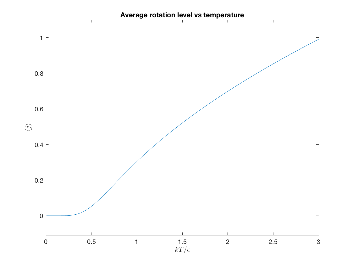
- What is the average value of \(j\) as a function of \(x\)?
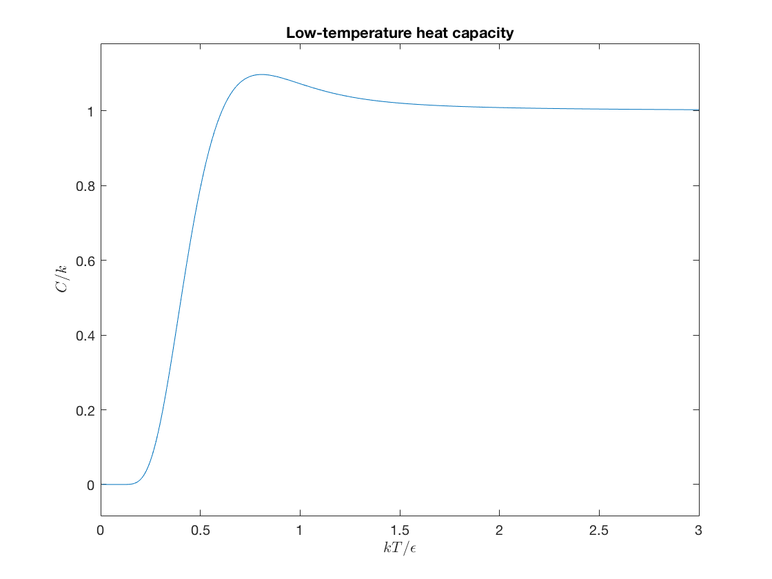
- Reproduce the following plot of the low-temperature behavior of the exact expression for the heat capacity. How does it compare to the expression one gets for the high-temperature approximation?
J=0:10; % Keep 11 terms
% define a vectorized version of the Boltzmann factor
boltz = @(x) exp( -(J.*(J+1))'./x ); % matrix / vector division
Z = @(x) (2*J+1)*boltz(x); % partition function
p = @(x) boltz(x)./Z(x); % probability of a *fixed* J, matrix / vector division
aveJ = @(x) (J.*(2*J+1))*p(x); % average J, including degeneracy term

ezplot(@(x) aveJ(x'),[0,3]);
title('Average rotation level vs temperature')
xlabel('$kT/\epsilon$','interpreter','latex');
ylabel('$\langle j \rangle$','interpreter','latex');
aveE = @(x) (J.*(J+1).*(2*J+1))*p(x);
aveE_sq = @(x) (((J.*(J+1)).^2).*(2*J+1))*p(x);
sigma_E_sq = @(x) aveE_sq(x)-aveE(x).^2;
heatC = @(x) sigma_E_sq(x)./(x.^2);

ezplot(@(x) heatC(x'),[0,3]);
title('Low-temperature heat capacity')
xlabel('$kT/\epsilon$','interpreter','latex');
ylabel('$C/k$','interpreter','latex');
Homonuclear diatomic molecules
In contrast to heteronuclear diatomic molecules, homonuclear diatomic molecules have a symmetry between the two atoms, so we must give them a more careful treatment.
When we count the degenerate number of energy levels for a homonuclear molecule, we must take into account that rotating the molecule by 180 degrees leaves the molecule completely unchanged. These are indistinguishable particles!
In fact, we can perform a detailed accounting of the allowed energies and their degeneracies if we know something about the spin of the atomic nuclei that comprise the molecule. The nuclei themselves can either have integer or half-integer spin, making them bosons or fermions respectivly. This constrains the total molecular state (wavefunction) to be either 'symmetric' or 'antisymmetric', and this in turn determines if we should sum over only odd or even values of j in the partition function so as to respect this symmetry.
We will get to bosons and fermions soon, and that will allow us to understand this symmetry at a deeper level. But for now we note that we must avoid double counting symmetric configurations. Thus, at least in the high-temperature limit, we can simply divide the partition function by a factor of 2 to correct for this symmetry. This is an approximation to the full and accurate accounting of the partition function that uses the nuclear spins, but it works well when \(kT\) is large compared to \(\eps\).
- How is the heat capacity affected by this factor of 2 in the high-temperature limit?
Maxwell Speed Distribution
The Maxwell speed distribution for an ideal gas is
\(\displaystyle \mathcal{D}(v) \mathrm{d}v = \Bigl(\frac{m}{2\pi kT}\Bigr)^{3/2} 4\pi v^2 \e^{-mv^2/2kT}\mathrm{d}v\)
Let's define this as a function. We first notice that \(m\) and \(kT\) always occur together. So the only thing that matters for the physics is this ratio. Therefore, we define a new variable \(u = \sqrt{2kT/m}\) and express the speed distribution in terms of this quantity. You'll recall from class that \(u\) is just the most probable speed of a particle. To make things dimensionless, which is convenient for plotting purposes, we'll introduce \(x = v/u\). Then the probability density as a function of \(x\) is
\(\displaystyle \mathcal{D}(x)\mathrm{d}x = \frac{4}{\sqrt{\pi}} x^2 \e^{-x^2}\mathrm{d}x \quad , \quad u = \sqrt{\frac{2kT}{m}}\quad , \quad x=v/u\,.\)
The Maxwell speed distribution is a good approximation to the true speed distribution in an ideal gas when the mass \(m\) is small compared to \(kT\), i.e. when \(u\) is large.
maxwell = @(x) 4/sqrt(pi)* (x.^2).*exp(-x.^2);
Remember the interpretation of this formula: the probability of finding a particle with velocity in the range \(v\) and \(v+\dd v\) is given by
\(\mathcal{D}(v) \dd v\,.\)
As a sanity check, let's make sure this integrates to 1 when we integrate over all speeds.
integral(maxwell,0,Inf)
ans =

    1.0000
Here's a plot of the speed distribution in these dimensionless units.
ezplot(maxwell,[0,4])
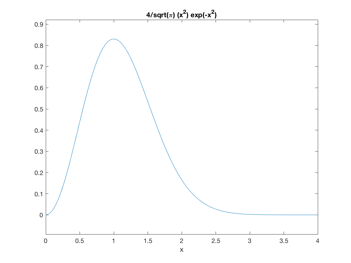
Again, we can visually check that the peak is at \(x=1\), meaning \(v=u\), as it should be.
Here is the first step in the derivation of the Maxwell speed distribution. We must compute the partition function. We can actually do this symbolically using the following commands.
% Define out variables
syms v m k T positive
% Define the integrand in the Partition function
% (degeneracy * Boltzmann factor)
z=4*pi*v^2*exp(-m*v^2/(2*k*T));
% Integrate to find the partition function
Z=int(z,v,0,inf);
% Output the dimensionful form
pretty(simplify(Z))
           3/2  3/2   3/2
2 sqrt(2) T    k    pi
-------------------------
            3/2
           m
Using the characteristic speed variable \(u\) introduced above, we can also simplify the result.
% Put in terms of the characteristic speed u
syms u positive
Z=subs(Z,T,m*u^2/(2*k));
% Output the new form
pretty(simplify(Z))
 3   3/2
u  pi
Of course, this integral can also be done with a change of variables and integration by parts, but it is nice to see that we can also do symbolic manipulations. The remainder of the derivation is left as an exercise.
Composition of the atmosphere
The Maxwell speed distribution can help us understand certain coarse features of our atmosphere.
The escape velocity of an object near the surface of the Earth is about 11 km/s. Particles traveling faster than this will leave the planet for good, assuming that they avoid any collisions on their way out.
In the thermosphere the temperature is actually quite high, more than 1000 K. (This is a bit misleading, because the atmosphere is so rarified at that altitude that a human would still freeze to death due to radiative heat loss before enough high-temperature gas particles collided with him or her.) At higher temperatures, energetic particles can reach higher speeds... but are these temperatures in the thermosphere enough for a particle to escape the clutches of Earth's gravitational field?
Let's see what will happen to a typical oxygen molecule in thermal equilibrium in the upper atmosphere. What is the probability that a randomly chosen molecule has a speed above the escape speed of 11 km/s?
kT = 1.38065e-23 * 1000; % Joules
mO2 = 2*16*1.66053892e-27; % atomic mass of oxygen molecule in kg
v_esc = 11000; % m/s, escape speed

u = sqrt(2*kT/mO2) % most probable speed in m/s

x_esc = v_esc/u % dimensionless escape speed;
u =

  720.8705


x_esc =

   15.2593
To escape, an oxygen molecule must be traveling more than 15 times the most probable speed, and 13.5 times greater than the average speed. Do we even need to compute the probability of escape? From the graph above, and the Gaussian decay of the Maxwell distribution, we can safely estimate that the fraction of escaping oxygen molecules is very close to zero.
integral(maxwell,x_esc,Inf)
ans =

  1.2963e-100
Yep. That's close to zero alright. Since there are fewer than \(10^{20}\) moles of oxygen molecules in the Earth's atmosphere, the probability that any of our oxygen is escaping due to temperature-induced speed fluctuations is totally negligable.
For hydrogen, it's another story. It is 16 times less massive than an oxygen molecule, so the most probable speed is 4 times greater.
mH2 = 2*1*1.66053892e-27; % atomic mass of hydrogen molecule in kg
v_esc = 11000; % m/s, escape speed

u = sqrt(2*kT/mH2) % most probable speed in m/s

x_esc = v_esc/u % dimensionless escape speed;
u =

   2.8835e+03


x_esc =

    3.8148
From the dimensionless escape speed, we can easily compute the probability that a hydrogen molecule has a large enough speed that it could escape.
integral(maxwell,x_esc,Inf)
ans =

   2.1276e-06
This is a small number, but nowhere near as small as for oxygen. It's clear that a substantial fraction of hydrogen molecules have left the Earth's atmosphere from this process.
The escape velocity of the moon is 2.4 km/s. What is the probability that an oxygen molecule will escape from the moon? (Assume a temperature of 1000 K still.)
v_esc_moon = 2400; % m/s, escape speed
u = sqrt(2*kT/mO2); % most probable speed in m/s
x_esc_moon = v_esc_moon/u; % dimensionless escape speed;

integral(maxwell,x_esc_moon,Inf)
ans =

   6.0169e-05
Now you should be able to explain: why does the moon have no atmosphere but the Earth does?