spaJS User Guide
Overview
spaJS is an interactive / data-driven / visual / online tool to conduct Structural Path Analysis (SPA). It has been developed from scratch and it is written in modern JavaScript (JS).
spaJS applies the technique of backwards scanning a network of transactions among the sectors in a given economy to retrieve all paths (or supply chains) which are deemed significant in terms of their contribution to the total impacts quantified by a given (environmental, social) indicator (or flow). Significant paths are defined in terms of a user specified threshold (or pruning) value relative to the total impacts, and are searched for up to a maximum order (or tier), also specified by the user.
spaJS features a simple, self-explanatory interface designed to guide the user step by step by enabling only those features that are appropriate for the chosen settings. spaJS has been inspired (*) by pyspa (written in Python) and the need for more freely available open source tools to conduct SPA.
spaJS is currently in its open beta version. We welcome feedback from the community, including suggestions for improvements, additions, bugs, etc. See Contact.
spaJS has been tried and tested in the following browsers:
- Chrome (recommended)
- Firefox
- Safari
(*) spaJS borrows some of the conventions adopted by pyspa, such as the names of some input files and their structure. The intent behind this is to allow the use of either tool with the same input data sets (subject to minor modifications).
spaJS comes with a fully functional Environmentally-Extended, Multi-Regional Input-Output dataset. Currently, this dataset consists of a compressed version of the full GLORIA (2018) dataset, referred to as GLORIA25, which spans 25 sectors across 164 regions, and one environmental indicator (green-house-gas emissions). The GLORIA25 dataset is available for download (zip format, 34 MB).
Did you know?
The OAASIS project and spaJS have been recognised with the Innovation Award at the 2023 Anti-Slavery Freedom Awards organised by Anti-Slavery Australia.
Features
spaJS allows to:
- Conduct SPA on extended Multi-Regional Input-Output (MRIO) data or on extended single-region data.
- Save the results as a list of paths in order of decreasing footprint (CSV format).
- Visualise the path hierarchy as a dynamic (interactive) tree diagram consisting of linked nodes.
- Visualise the commercial links between the consumer country and its suppliers on a World map
Limitations
- SPA is conducted on one sector and one indicator at a time.
- The default dataset is limited to a handful of sectors and only one environmental indicator (see Overview).
- spaJS allows for alternative input datasets from the user, but the size the user input dataset is currently limited to ~300 MB.
Usage
The workflow with spaJS can be broken down into three stages:
These stages are explained in turn. Please consult our adopted definitions and conventions. All the examples that follow are based on a dummy dataset and are only relevant for the purpose of illustration.1. Data Input
User Input Data
spaJS requires the user to upload four input text files in comma-separated-value format (CSV):
- A_matrix.csv: The content of the intermediate demand matrix \( A \)
- Infosheet.csv: This file contains information about the regions and their sectors.
- Intensities.csv: This file provides the direct impacts (or requirements) \(q\) and the total impacts (or requirements) \(m\) for each of the indicators for each sector in each region.
- Input.csv: This file provides the total output (\(x\)) and total final demand (\(y\)) for each sector in each region.
The required files are uploaded one by one via the upload buttons (Screenshot 1.1).
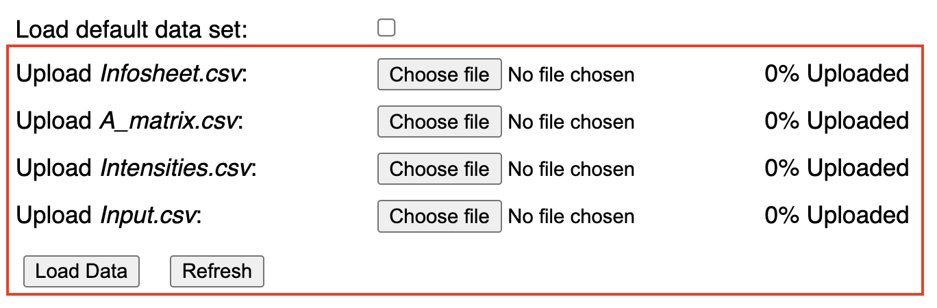
Note that the files must be named as shown to the left of each button. This quirk is intentional in order to avoid the user from potentially uploading the wrong file, e.g. an Input.csv file where a A_matrix.csv file is expected. Note that the files are not checked for content other than their size, e.g. A_matrix.csv is expected to containt \( N + 1 \) rows (see above) and \( N \) columns; in turn, all other files are expected to contain \( N + 1 \) rows. If any of these conditions is not met, spaJS will display a browser alert.
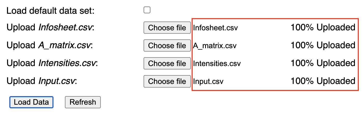
After choosing a file, its name appears next to the corresponding upload button and the field next to it indicates that the file has been fully (100%) uploaded (Screenshot 1.2). To load the file data onto the browser's memory, simply click the button. To clear all the chosen files, press the button. Note that the data can be loaded onto memory only upon uploading all required files.
Default Input Data
As an alternative to the option to load custom input files, spaJS provides a built-in default dataset: The GLORIA25 dataset, a compressed version of the full GLORIA (2018) dataset, which spans 25 sectors across 164 regions, and one environmental indicator (green-house-gas emissions). The GLORIA25 dataset is available for download (zip format, 34 MB).
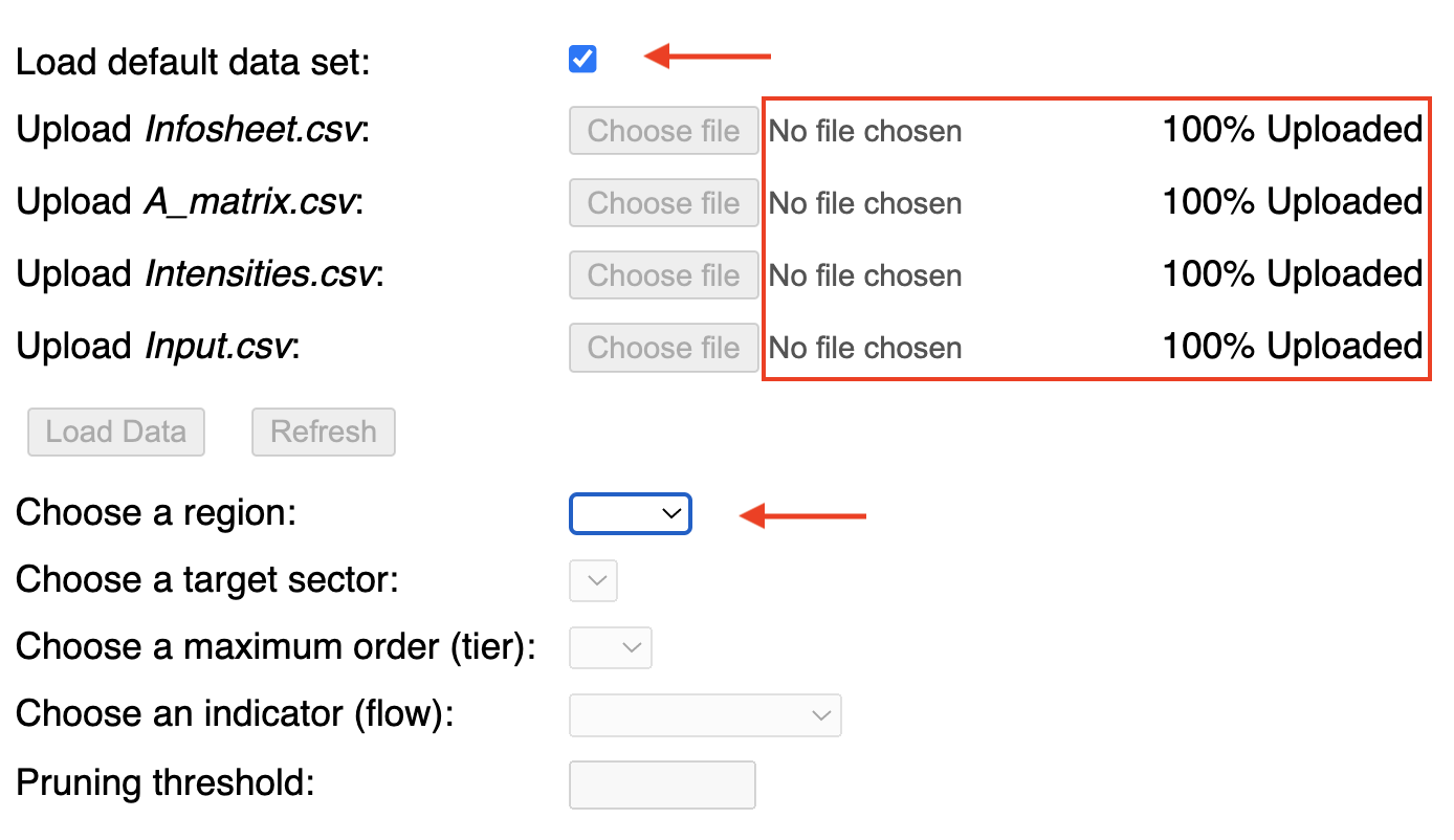
To directly load the built-in default data set, simply check the box at the top of the interface. The user upload interface is disabled, and once all files have been automatically loaded, the user is directed (via element focusing) to the relevant input menus, starting with the 'Choose a region' menu (Screenshot 1.3). Note that in this case, the file name is not indicated next to the corresponding button, but the field next to it does indicate that the file has been fully loaded (compare to Screenshot 1.2).
For slow internet connections, we recommend downloading the default dataset to disk and then load it via the user input interface as explained above, rather than loading it directly as a default data set.
2. Scanning Parameters
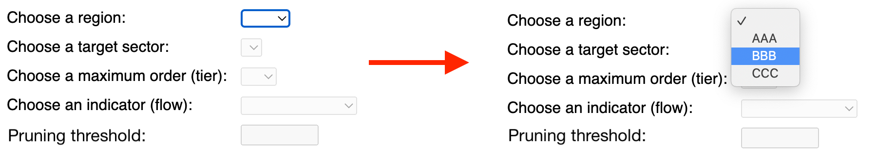
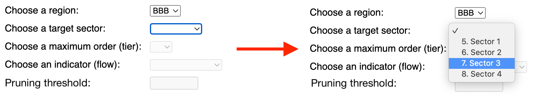
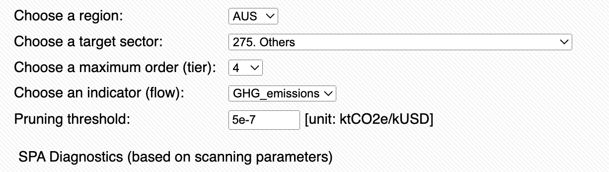
Once the input data is loaded onto memory, the input menus and input fields that define the scanning parameters (region, sector, order, indicator, pruning threshold) are automatically populated, although only the 'Choose a region' menu is enabled at this point (Screenshot 2.1, left). For the sake of illustration, here we will use a dummy data set, consisiting of four fictitious sectors across three fictitious regions (AAA, BBB, CCC). The user is asked to:
- Select a region from the menu; the menu is automatically populated with all the unique alpha-3 code regions as given in file Infosheet.csv (Screenshot 2.1). This action enables the subsquent input menu.
- Select a target sector from the menu; the menu contains all the unique sectors included in file Infosheet.csv (Screenshot 2.2). This action activates the subsquent input menus.
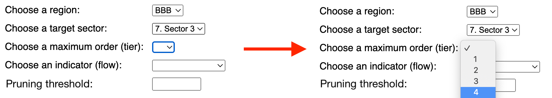
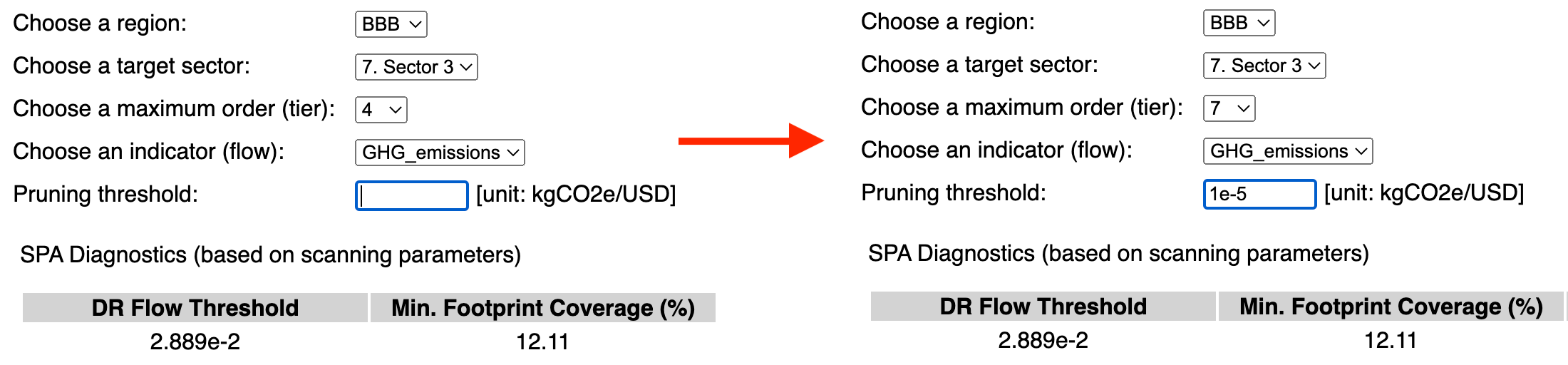
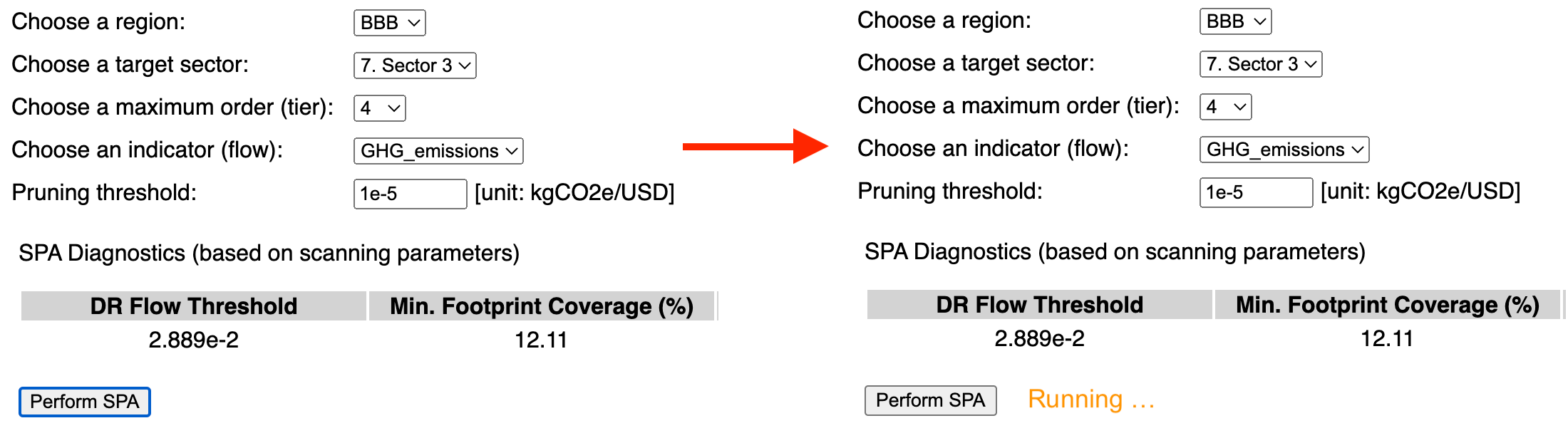
- Set a maximum order (Screenshot 2.3). Note that the maximum order is limited to 10 for the time being, which should be sufficient for most applications (it can be increased upon request). Here we chose 4. Generally, however, it is always a good idea to start with a low value, e.g. 2, and then increase it, since the number of signficant paths will generally increase (exponentially) with increasing order value. The same applies for the pruning threshold (see below).
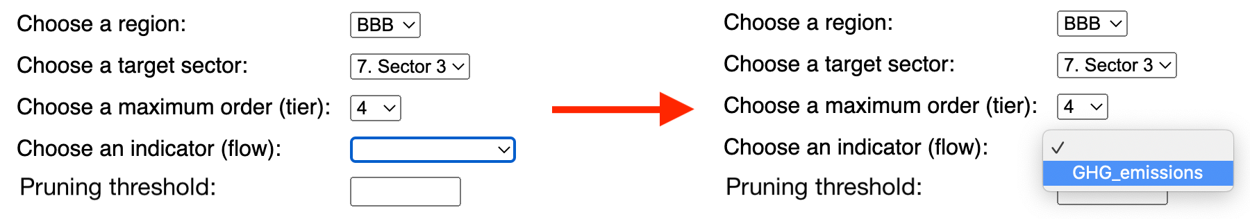
- Select an indicator (Screenshot 2.4a). The menu is populated with all the indicators included in file Intensities.csv. In this case there is only one, 'GHG_emissions'.
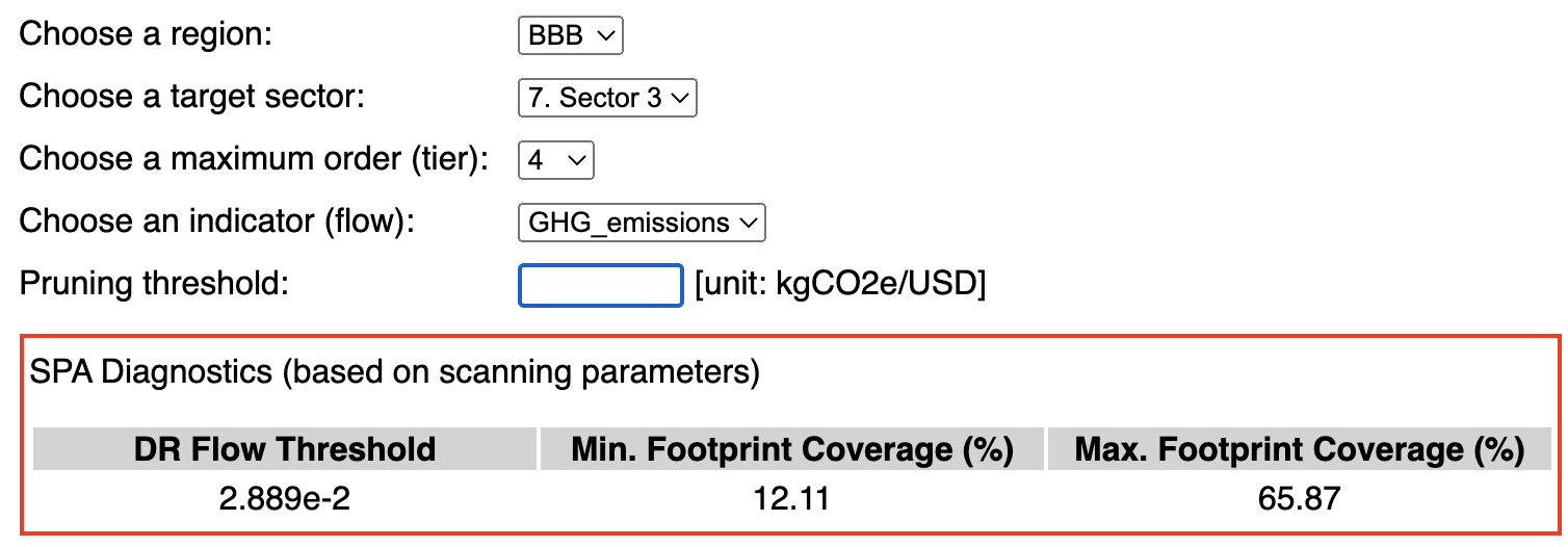
- Set a pruning (threshold) value (Screenshot 2.5). In general, the lower the threhsold value, the more paths will be found. The maximum (meaningful) pruning value is defined by the DR value given in the 'SPA diagnostics' table (Screenshot 2.4b, left column). If the threshold is set to a value equal or higher than this, only one path, namely the direct stage (on-site) will be found. In this case, the total coverage of the network will correspond to the minimum footprint coverage given in the 'SPA diagnostics' table (Screenshot 2.4b, central column). Lower pruning values will generally lead to a larger number of significant paths. If the pruning value was set to 0, then all paths up to the selected order will be scanned for. The total coverage of the network will correspond to the maximum footprint coverage given in the 'SPA diagnostics' table (Screenshot 2.4b, right column). In general, such a practice is discouraged as the number of paths may be too large and this may overload the browser. Meaningful pruning values are typically much smaller than 1, but not 0, (for example, 0.0001). That said, it is always a good idea to start with a value close to (but smaller than) the value indicated in 'SPA diagnostics' table under 'DR Flow Threshold', and then progressively decrease it, since the number of signficant paths will generally increase (likely exponentially) with a decreasing threshold (pruning) value. The same applies for the maximum order (see above). Note that values can be entered using exponential notation (e.g. 1.0e-3 or 1e-3) or decimal notation (0.001). In this example, we set the pruning threshold to 1e-5.
- If all settings are correct (i.e. all menus have a selected value and the threhsold value is valid), the button is enabled. Pressing this button starts the process. A flashing message 'Running...' appears next to the button to inform the user that the calculation is running, and it disappears when the process has completed (Screenshot 2.6)
Once a flow has been chosen, spaJS performs two tasks: 1) It updates the 'Pruning threshold' field by adding the appropriate unit to the right (the unit is adapted from the information provided in the Intensities.csv file); in this case, it is 'kgCO2e/USD', or 'kilogram of equivalent CO2 emission per US dollar'. 2) It calculates the flow value of the direct impact (or requirement, DR), as well as the minimum and maximum footprint coverage which are consitent with the values of region, sector, and order. This information is diplayed on a table called 'SPA Diagnostics', displayed right below the scanning parameter input fields (Screenshot 2.4b). The minmimum and maximum footprint values indicate the minimum and maximum coverage (in percent, relative to the total coverage) of the supply chain network defined by the region, sector, and flow. The minimum corresponds to the footprint of the direct stage (i.e. on-site), while the maximum corresponds to the footprint of the entire network up to the order set (in this example, 4). Thus, the latter will never reach 100% (unless the order is set to infinity), but may reach close to 100% depending on the characteristics of the supply chain network. The flow value corresponding to the direct impact (or requirement, DR) indicates the maximum (meaningful) threshold value above which no paths other than the direct path will be found (see below).
3. Save / Visualise Results
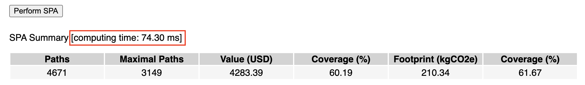
Upon completing the scanning, spaJS displays a summary of the results in tabular form (Screenshot 3.1). The table informs the user about: (1) the total number of significant paths compatible with the scanning parameters; (2) the number of maximal paths (see Definitions); (3) the aggregated monetary value and its coverage relative to the target sector's \( x \); (4) the aggregated footprint and the its coverage with respect to the target sector's \( m \). In this context, 'aggregated' refers to the result of adding up the corresponding flow quantity for all retrieved paths. The units of the value and of the footprint correspond to the monetary units and the indicator units as given in the file Infosheet.csv. Note that the footprint coverage is always less or equal than the maximum footprint coverage indicated in the 'SPA diagnostics' table (Screenshot 2.4b, right column), as it should.
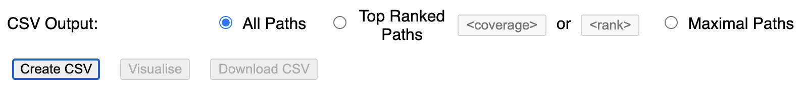
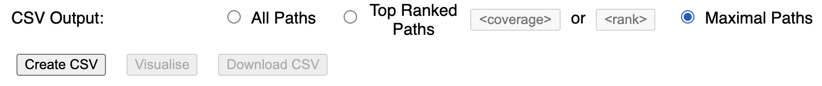
The next step is to cast the results into a CSV structure containing the paths ranked in order of decreasing footprint which can be downloaded as CSV file or visualised (or both). This is done simply by clicking the button (Screenshot 3.2, top). By default, spaJS includes all paths (4671 in this example; see Screenshot 3.1); thus the 'All paths' radio button is checked by default. However, the user is given the choice to select only a subset of paths. The subset can be defined either in terms of footprint coverage or in terms of ranking (paths are ranked in decreasing order of footprint). The footprint coverage is entered as a percentage, with possible values between 0 and 100, e.g. 50., while the rank is entered as an integer number \( p\) between 1 and the total number of paths (in this example 4671), e.g. 15, indicating the wish to select only the first \( p \) top-ranked paths from the list. Either of these is achieved by checking the 'Top Ranked Paths' radio button and entering the value of the coverage or \( p \) in the corresponding field, and pressing the <enter> key (Screenshot 3.2, middle-top, middle bottom). Alternatively, the user may choose to select only the maximal paths by checking the 'Maximal Paths' radio button (Screenshot 3.2, bottom). Note that if no maximal paths are found, this button is disabled.
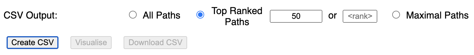
![]()
Once the choice has been made among either all paths, the paths with a specified coverage, the \( p \) top-ranked paths, or the maximal paths (if available), the CSV structure is created by pressing the button (Screenshot 3.2, bottom, shown in focus). This action triggers two subsequent actions: (1) it enables the 'Visualise' and the 'Download CSV'; (2) it displays a sample of the path list in tabular form (Screenshot 3.3). In this example, we have chosen to include only the 15 top-ranked paths.
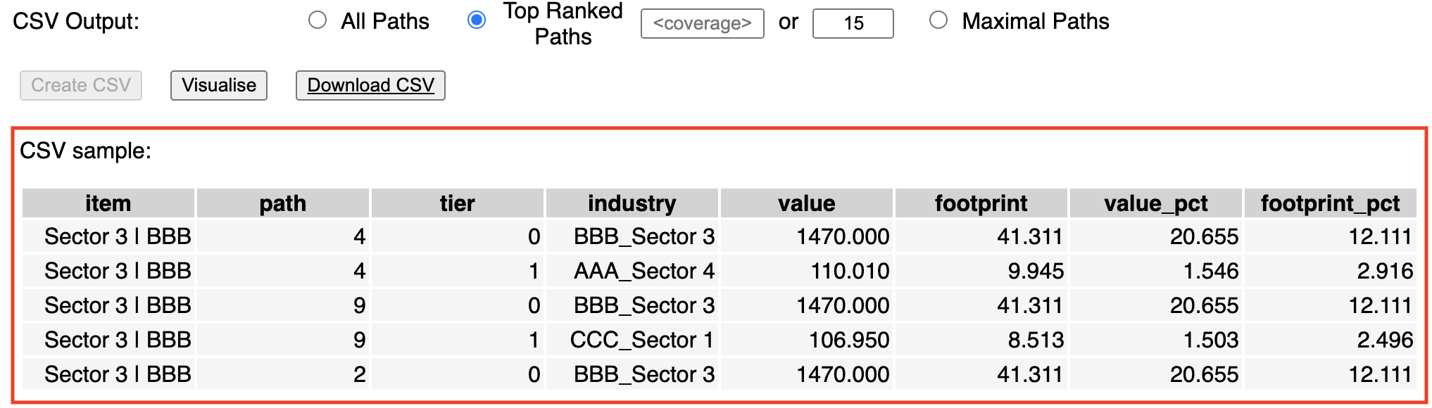
- item (type string): A concatenation of the target sector's name (downstream endpoint) and its corresponding region, e.g. 'Sector 3 | BBB'. Its value is identical for all entries in the table.
- path (type integer): An ID assigned to each path. Paths along a common 'branch' of the tree hierarchy are assigned the same ID (see Visualisation).
- tier (type integer): The order (or tier) of the path
- industry (type string): A concatenation of the upstream endpoint sector's name and its corresponding region, e.g. 'BBB_Sector 3'.
- value (type float): The value of the path in the monteary units provided in the Infosheet.csv
- footprint (type float): The footprint of the path for the chosen indicator, in the units provided in the Infosheet.csv
- value_pct (type float): The value coverage of the path in percent relative to the target sector's \( x \)
- footprint_pct (type float): The footprint coverage of the path in percent relative to the target sector's \( m \)
Saving the results
Saving the results to a CSV text file is as easy as pressing the button, which in turn opens an operating-system dependent file save dialog, and the user is asked to choose a location and a enter a name; spaJS provides the default name 'spajs.csv'. We recommend adding information about the scanning parameters to the file name in a prescribed order, e.g. 'spajs_<maxorder>_<indicator>_<threshold>.csv', since such information is not included in the file (this shortcoming will be addressed in future versions of the tool).
The file content consists of the path list in CSV format following the same structure as provided by the sample table (Screenshot 3.3). The paths are ranked in decreasing order of footprint. Note that the path ID does not reflect in anyway their ranking!
N.B.: All the entries with a tier value of 0 are identical in every aspect with exception of the value in the 'path' column. This quirk is a remnant of previous (unreleased) versions of the tool, and it may dissapear in the future.
Visualisation
Tree structure
Once a CSV structure has been created, in addition to save the results to disk it is possible to visualise these directly in the browser.
spaJS provides an interactive visualisation using a dynamic tree hierarchy where the sectors along the retrieved paths are represented by nodes and their transactions by links. In this hierachy, the target sector ('item' in the above sense) sits at the root node (to the left of the tree), while upstream suppliers ('industries' in the above sense) are located along 'branches' of the tree (extending to the right of the root node).
A node sitting on tier \(\tau \) is said to be 'parent' to a linked node sitting on tier \(\tau + 1\). Conversely, a node sitting on tier \(\tau + 1\) is said to be a 'child' of a linked node sitting on tier \(\tau \).
When displaying the tree hierarchy, nodes along paths which are identical in every aspect except for their ID are 'zipped' together to avoid redundancy at each tier. For instance, even though all entries in the CSV structure identified by an unique ID share the same root node, the latter is displayed only once. Thus a set of \( k \) linked nodes (where \( k = 1, 2, ... \) ) represents \( k \) different paths of order 0, ..., \( k - 1 \).
Note that although the paths are ranked in order of decreasing footprint in the CSV structure (and consequently in the downloadable CSV file), that may not always be the case in the tree visualisation as a result of the 'zipping' of common paths (see above). In other words, the top-bottom structure of the tree branches does not need reflect the paths' ranking. For ease of identification, the top-ranked path is explicitly highlighted, and each path's rank is displayed upon hovering (see below).
Visualising the results is to a CSV text file is achieved by pressing the button. This action opens a new DOM area below the CSV Sample table, displaying the tree hierarchy and preceeded by an information panel.
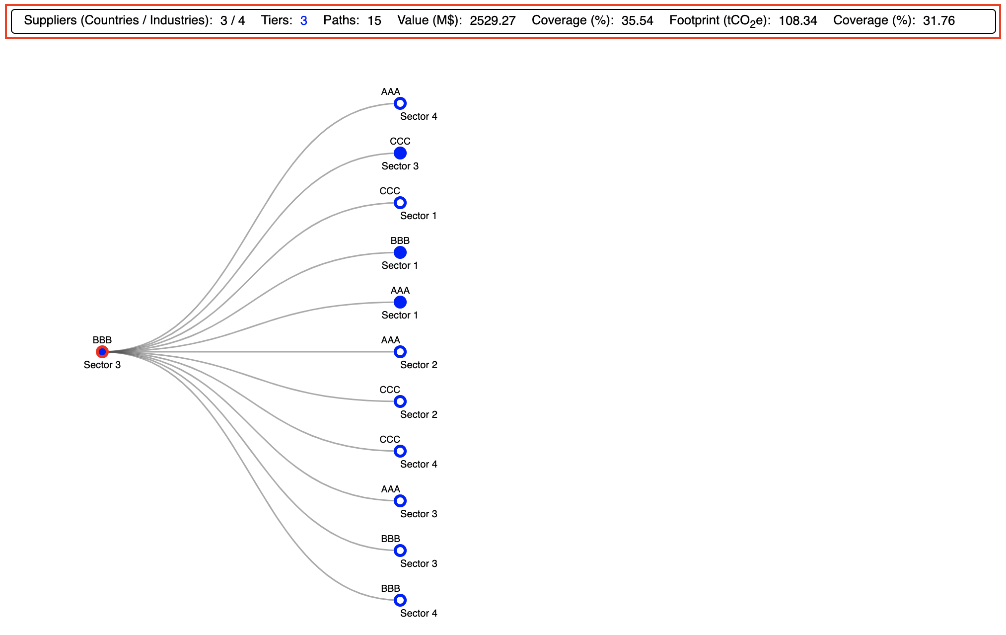
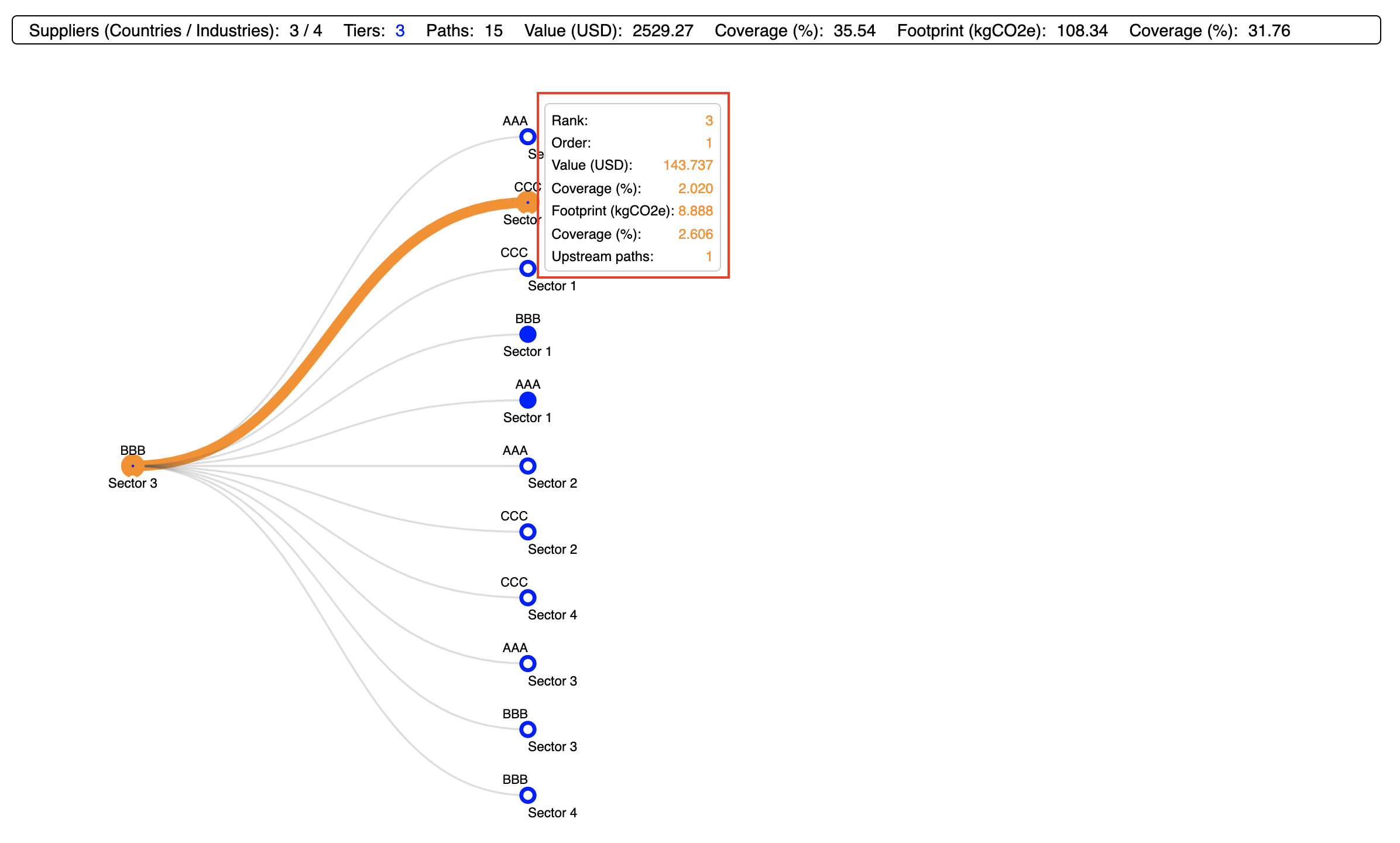
The information panel (Screenshot 3.4, highlighted in red) presents a summary of the CSV structure data (i.e. of the visualised data); it displays the following:
- The total number suppliers split by sectors and countries
- The number of tiers. Note that this number does not necessarily matches the maximum tier scanned for (see Scanning Parameters) if there are no maximal paths in the (top-ranked) path list.
- The number of paths. Note that this number will only match the corresponding number in the SPA summary if all paths have been included in the CSV structure. If paths have been selected in terms of coverage, the displayed number will be smaller than the total number of paths, unless the coverage is equal to the maximum coverage given in the table 'SPA Diagnostics'. If instead the \( p \) top-ranked paths have been selected, then the number displayed here may be equal or higher than \( p \). The latter case arises when a path among the \( p \) top-ranked lies along the branch of a path at a lower tier which is not contained within the \( p \) top-ranked.
- The aggregated value and its coverage. Note that these numbers will only match the summary presented in the SPA summary if all paths have been included in the CSV structure (Screenshot 3.2, top). Otherwise they will always be smaller.
- The aggregated footprint and its coverage. Note that these numbers will only match the summary presented in the SPA summary if all paths have been included in the CSV structure. Otherwise they will always be smaller.
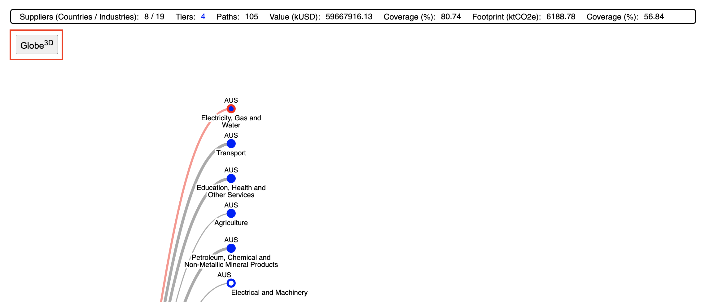
The tree (Screenshot 3.4, bottom) is displayed with the root node on the far left, and all the paths (nodes) extending to the right. Initially, only paths extending to tier 1 (i.e. of order 1) are displayed. The tree itself provides a wealth of information:
- Each node represents a path (or supply chain), and each is accompanied by its corresponding region and corresponding sector name
- Each sequence of \( M \) linked nodes represents a path of order \( M - 1 \) (see below).
- The link corresponding to the path with the highest footprint (i.e. the number 1 top-ranked) is highlighted in red. In the above example, it is the direct path of the sector, thus the root node is highlighted (Screenshot 3.4, bottom)
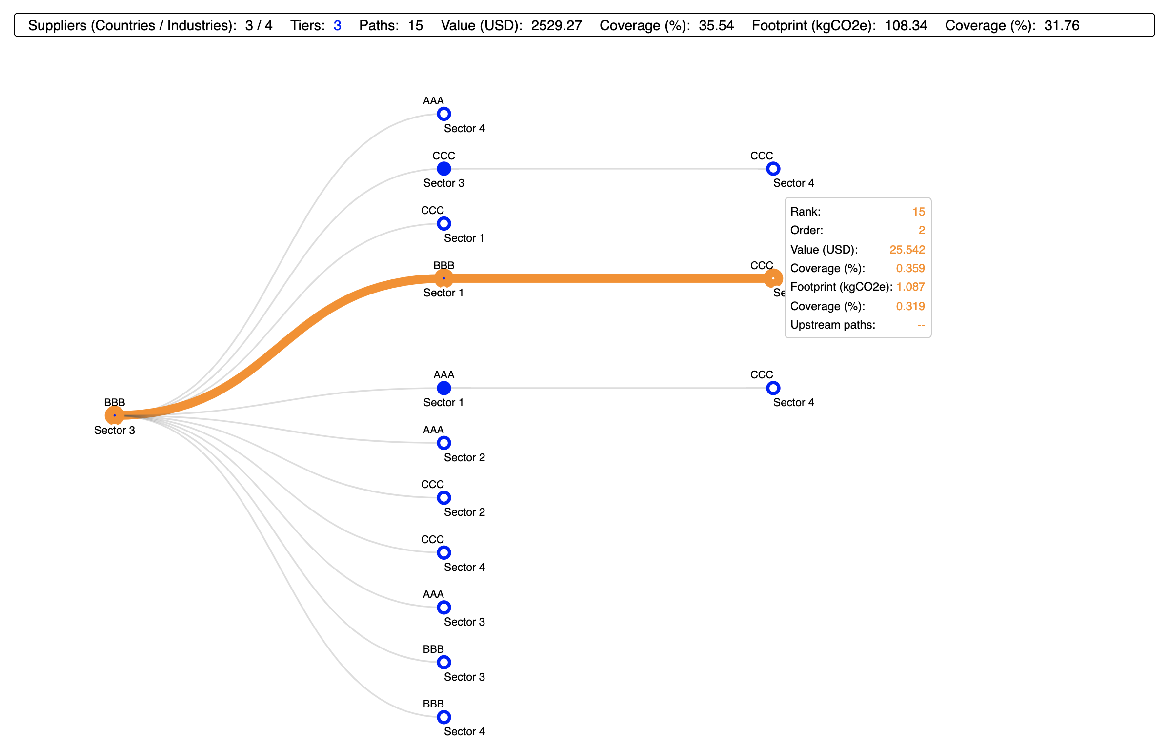
- Hovering over a node results in its corresponding downstream path being highlighted in orange, and a tooltip being displayed, with the following information: path rank and order, value and coverage, footprint and coverage, and number of upstream paths linked to the node (Screenshot 3.5, Screenshot 3.7)
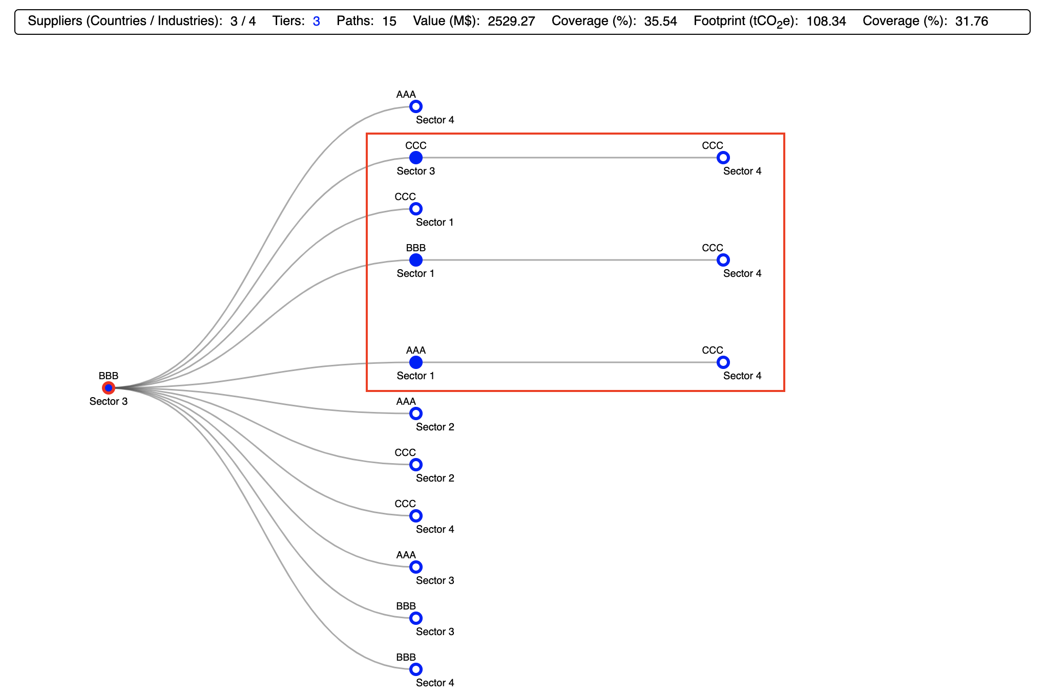
- The width of the link between nodes is loosely indicative of the number of upstream paths linked to the child node (this feature may be replaced by a qualitative relationship between width and path footprint).
- All upstream end point nodes are shown as open circles; filled circles indicate the existence of upstream paths. Clicking on a 'full' node displays all the linked paths one tier upstream (Screenshot 3.6)
Note that the viewport's height is dynamically adjusted as required in response to displaying an increasing number of paths at higher tiers (i.e. by clicking on 'full' nodes). This is relevant because it allows to display a large number of paths even if they do not fit into the screen.
NEW
World map
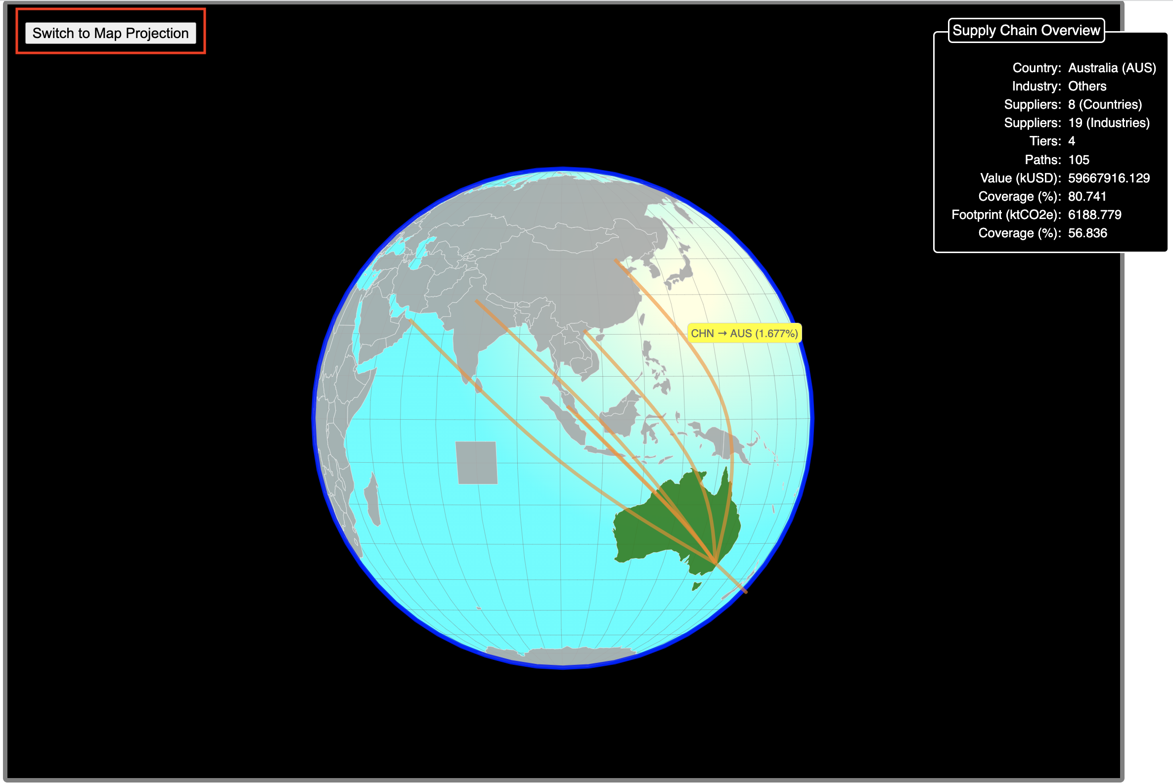
In addition to the rather abstract tree visualisation, spaJS alows to visualise the commercial links between the consumer country and its suppliers (all tiers, all sectors) geographically. The default visualisation is based on a D3 interactive, pseudo-3D globe. In order to access the 3D globe, simply press the located just below (and to the left of) the information panel of the tree visualisation (Screenshot 3.9; this button was not available in previous spaJS versions and is therefore absent in comparable screenshots). Note that in the following we will use a supply chain example based on the default input data (rather than on a dummy data set as before). The scanning parameters in this example are indicated in Screenshot 3.8
The 3D globe projection is initially centred on the consumer country, highlighted in green colour. Each of the links to its suppliers (all tiers, all sectors) is indicated as an arched, orange line ending on the corresponding supplier country. Hvering over any country indicates its name and ISO-3166 3-letter code. Hovering over any link reveals the supplier and cosunmer countries joint by an arrow, and the value of the total footprint of the economic activity between these countries over all tiers and all sectors. Note that the link between the consumer country with itself is indicated by a vertical line. The 3D globe representation in addition offers a summary view of the consumer country's supply chain, in the form of an information panel located to the top-right corner (Screenshot 3.10). The information there is equivalent to the information given in the top panel above the tree structure (Screenshot 3.4). Crucially, the Globe can be rotated in any desired direction by click-and-drag to reveal the full extent of the links.
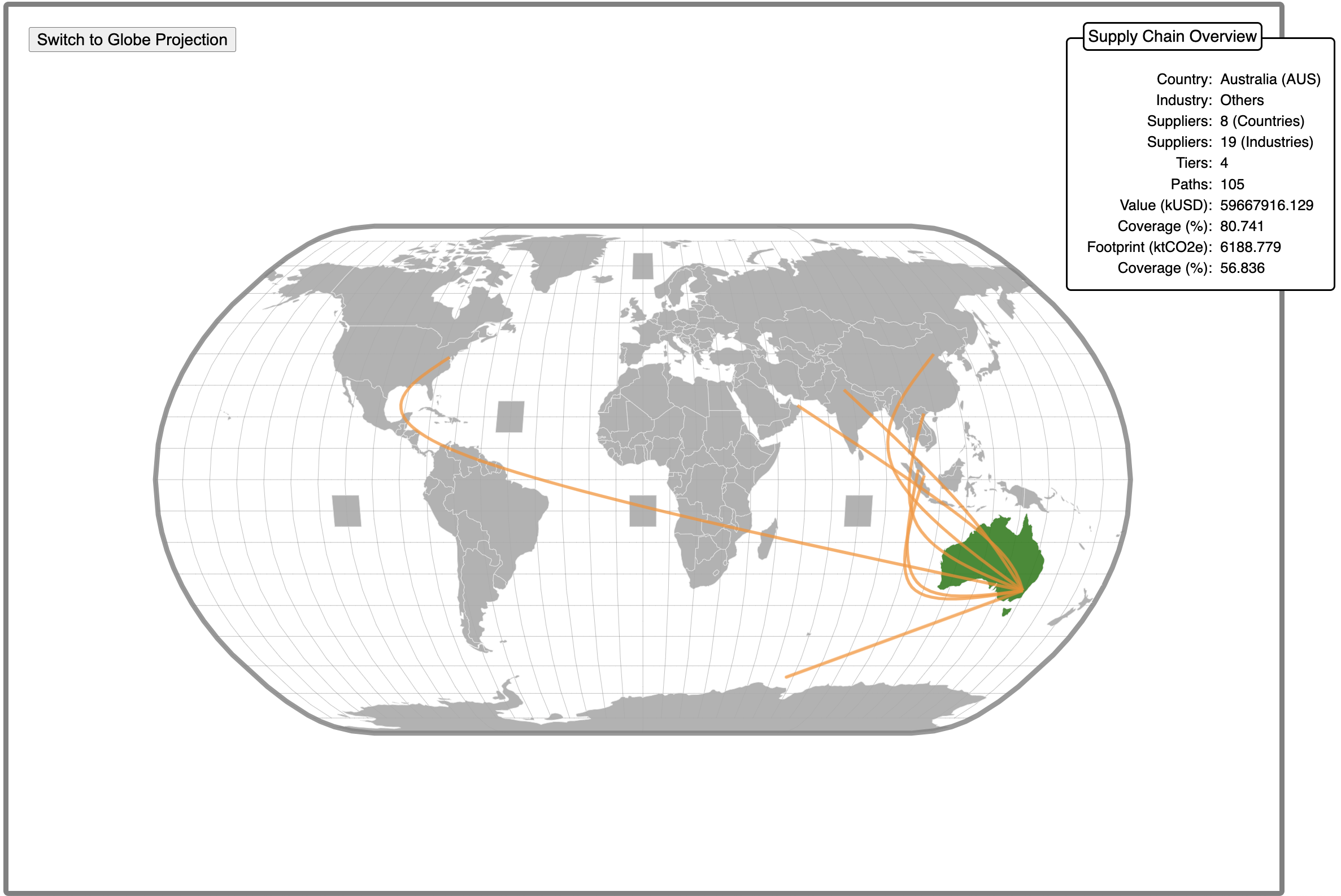
Alternatively, the globe can be projected onto a 2D (Natural Earth) map. This is achieved by pressing the located at the top-left corner of the Globe projection (Screenshot 3.10, highlighted within a red rectangle). All the features of the 3D globe are also avaible in the 2D projection (with exception of the rotation feature). Also, when projected onto 2D, the map is conventionally centred on the mid Atlantic ocean. Furthermore, the 2D representation shows at a glance the entire set of links between the consumer country and its suppliers (Screenshot 3.11). This representation is useful to generete a graph that can be used in, e.g., a report. For this reason, the projection adopts a different colour scheme compared to the Globe projection. Note that the option to save (or print) the map projection shall be implemented in future versions of spaJS.
Input File Structure
The required structure of each CSV input file is detailed in the following. See also the notes on file sizes.
A_matrix.csv
This file holds the entries of the \( A \) matrix arranged in columns and rows. The first row contains the indices of the columns, starting from 1. Thus, if \( A \) is of size \( N \times N \), the file must contain \( N + 1 \) rows. Note that this file shares an identical structure to the homonymous file required by pyspa.
The following is a downloadable example: A_matrix.csv.
Infosheet.csv
This file contains four columns with the following headers: SectorID, Name, Unit, Region.
The entries under 'SectorID' must match the column headers of A_matrix.csv. 'Name' corresponds to the sector's name. 'Unit' refers to the monetary unit of the economy considered, e.g. AUD. Note that multipliers, e.g. millions, thousands, should be specified by providing the appropriate prefix: MAUD, kAUD, etc., respectively. 'Region' denotes a country or region, preferably identified by its ISO-3166 alpha-3 code, e.g. AUS for Australia. If such a code is not available, a short name should be provided, e.g. 'Congo' rather than 'Democratic Republic of Congo', or 'RoW' rather than 'Rest of the World'. The first four columns of this file are identical to the homonymous file required by pyspa.
The following is a downloadable example: Infosheet.csv.
Intensitites.csv
This files contains at least three columns with the following headers: SectorID, DR_aaa_(bbb), TR_aaa_(bbb)
The entries under 'SectorID' must match the column headers of A_matrix.csv. 'DR' correspond ot the direct impacts (or requirements) \( q \), while 'TR' corresponds to the total impacts (or requirements) \( m \) of a given indicator (flow). 'aaa' gives the indicator name, e.g. "GHG_emissions", and 'bbb' specifies the unit, e.g. kgCO2e. Note that, strictly speaking, the units should be, e.g. kgCO2e/AUD, but this is implicitly acknowledged. This file may hold one or more indicators, as long as they are provided next to each other following the structure indicated above, i.e.:
SectorID, DR_aaa_(bbb), TR_aaa_(bbb), DR_ccc_(ddd), TR_ccc_(ddd) [, ... ]
Note that each DR_*** column must be followed by its corresponding TR_***. It is worth noting that the columns in this file follow the same structure as columns 5+ in the Infosheet.csv file file required by pyspa.
The following is a downloadable example: Intensities.csv.
Input.csv
This file contains thre columns with the following headers: SectorID, Stressor_Y, X_Out
The entries under 'SectorID's must match the column headers of A_matrix.csv. 'Stressor_Y' correspond to the total final demand (or stressor) \( y \) for each sector in the units specified by 'Unit' in the Infosheet.csv file. 'X_Out' corresponds to the total output (or input) \( x \) in the units specified by 'Unit' in Infosheet.csv.
The following is a downloadable example: Input.csv.
Notes on file sizes
spaJS has been succesfully tested with a number of sectors of up to \(N = 5000 \), or equivalently a total file size of up to 300 MB. In such cases, loading the required data takes on the order of 10-20 seconds depending on the browser and the available internet connection. Although it may be possible to handle larger files, this is yet to be tested. Note that file sizes can be significantly reduced by expressing their numerical content using scientific notation and reducing the number of significant figures, e.g. 1.23e-5 rather than 0.0000123024. Obviously, this does not apply to integer numbers, such as the sector ID or the headers of A_matrix.csv. Needless to say, reduced file sizes may allow to handle a larger \( N \) more efficiently.
Performance
spaJS has been put to the test using pyspa as benchmark. Using pyspa's template input data (version 06 MAY 2019), we have timed several SPA calculations with both pyspa and spaJS on a Mac Book Pro 2020 (macOS Catalina). spaJS has been tested in three different browsers: Chrome, Firefox, and Safari. While the results obtained with either code perfectly agree with one another for each given set of scanning parameters, there are significant differences in terms of speed. These are summarised in Table 1. Note that speed-up values larger than 1 imply a faster calculation, i.e. a better performance.
| Browser | Speed-up |
|---|---|
| Chrome | 7x |
| Firefox | 1.5x |
| Safari | 0.5x |
Requirements
- An ECMAScript 2019 compatible browser
- An active internet connection (not possible to use offline)
Bugs
The following is a list of known bugs to be adressed in future versions of the tool.
- The CSV output file may not be strictly in decreasing order of footprint if the branch with ID = 0 is associated with other path(s) in addition to the direct path (root node).
Contact
→ Send feedback, comments, suggestions, bug reports, ...
Acknowledgements
spaJS has been developed as part of the Open Analysis to Address Slavery in Supply Chains (OAASIS) project led by Joy Murray, generously funded by the Physics Foundation at The University of Sydney through a Physics Grand Challenge grant. We acknowledge the use of the Eora database in the early stages of spaJS’s development.
The GLORIA25 dataset has been put together by Jacob Fry and Arunima Malik, using resources from the Industrial Ecology Virtual Laboratory (IELab).
The development of spaJS would not have been possible without the wealth of technical support provided by, among others: the Stack Overflow forum; the official documentation of HTML, CSS, and JavaScript provided by the Mozilla Developer Network (MDN) and W3 Schools; the existence of freely available JS libraries, in particular Mike Bostock's D3 and Jos de Jong's mathjs; and free powerful editors such as Atom.
Special thanks to André Stephan and Rob Crawford for the development of and their assistance with pyspa, a code that inspired spaJS.
Please acknowledge the use of this software by referring to Tepper-García et al. (2021).
Built with ...
spaJS has been written in modern JavaScript (ECMAScript 2019). It takes advantage of the power of mathjs and D3. It has been developed and tested with the Atom editor and its atom-live-server package.
Definitions
For the sake of clarity, we adopt the following definitions and conventions.- \( N \) refers to the total number of sectors across all regions. For example, it there are \( p \) sectors in \( k \) different regions, then \( N = p \times k \).
- \( A \) is the intermediate demand matrix (or production recipe) of size \( N \times N \).
- \( x \) corresponds the total output (or total input), and \( y \) to the total final demand; these are both vectors of size \( N \).
- \(q\) corresponds to the direct impacts (or requirements); it is represented in general by a matrix of size \( M \times N \), where \( M \) is the number of indicators (\(M\) can be 1).
- \(m\) corresponds to the total impacts (or requirements) given by \( m = q L \), where \( L = (I - A)^{-1} \) is the Leontief inverse. \( m \) is represented in general by a matrix of size \( M \times N \), where \( M \) is the number of indicators (\(M\) can be 1).
- A path from the upstream sector \( i \) down to the target sector \( n \), abreviated \( i \to n \), is a sequence of the form \( q_i \, A_{ij} \ldots\, A_{mn} \,y_n \); it is also referred to as a 'supply chain'.
- The order of a path is the number of \( A \) factors in the sequence \( q_i \, A_{ij} \ldots\, A_{mn} \,y_n \); its values matches the path's tier. It is also commonly referred to as stage or layer.
- A path is said to be maximal if its order is equal to the maximum order scanned for (see Scanning Parameters)
- The rank of a path corresponds to its position in a list of paths organised in decreasing order of footprint.
- The value of a path \( i \to n \) is given by \( V_{i \to n} \equiv A_{ij} \ldots\, A_{mn} \,y_n \), while its footprint as measured by indicator \( j \) is given by \( F_{j,i \to n} = q_{ji} V_{i \to n} \).
- The downstrem end point of a path is given by the sector sitting at the tier 0. For example, if a path is \( q_i \, A_{ij} \ldots\, A_{mn} \,y_n \), the downstream end point is \( n \). It is equivalent to the target sector (also referred to as 'consumer').
- The upstream end point of a path is given by the sector sitting at the highest tier. For example, if a path is \( q_i \, A_{ij} \ldots\, A_{mn} \,y_n \), the upstream end point is \( i \).
disclaimer
spaJS is free software that is provided as is, and comes without any warranty of any kind.
license
The use of this software is governed by a creative commons attribution non-commercial license. Note in particular that this license prohibits the use of this software for any commercial purposes.
Please acknowledge the use of this software by referring to Tepper-García et al. (2021).