![[Square compound double pendulum]](sdpend_figure/sdpend_model.jpg)
The equations of motion may be determined from the Lagrangian.
The kinetic energy of the device is the sum of the translational kinetic
energy of the centre of mass of each plate, and the rotational kinetic
energy of each plate about its centre of mass. The potential energy is
equivalent to that of two point masses at the locations of the centre of
mass of each plate. The equations of motion (for equal mass plates) are:
![[Square compound double pendulum]](eom_sdpend.jpg)
and where g denotes the acceleration due to gravity. The equilibrium
configuration is obtained by setting the time derivatives to zero. This
leads to
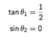
which has four solutions, only one of which corresponds to a stable
equilibrium configuration. The stable equilibrium is when the diagonal
of the top plate is angled by about 26.6 degrees, and the bottom plate
hangs straight down. (It is easy to confirm that this implies zero net
torque about the two pivot points.)
The equations may be rewritten as four coupled first order ODEs, and then numerically solved using standard methods. It is helpful to non-dimensionalise by scaling time in units of the square root of L over g. The C code used to solve the equations is here. The method of integration is fourth order Runge-Kutta. No explicit checking on accuracy is performed, but the energy is calculated at each time step.
The equilibrium configurations provide simple checks on the implementation of the equations. The movie on the left below shows the system evolved starting at the stable equilibrium in which the diagonal of the top plate is angled by about 26.6 degrees, and the bottom plate hangs straight down. The movie at right below shows one of the unstable configurations, which is the inverted version of the stable configuration. The numerical solution reveals the instability - the top plate falls down eventually.