Low energy

At low energy, the pendulum exhibits small oscillations about the stable equilibrium. There are two strictly periodic normal modes of oscillation, which may be demonstrated in the real pendulum by turning the handle at the correct frequency for each mode. The animations below illustrate the fast normal mode (on the left), and the slow normal mode (right). In the fast mode the plates oscillate in opposite directions, and in the slow mode they oscillate in the same direction. The animations also show the centre of mass of the outer plate (the cross) and the equilibrium position of the lower plate (the vertical dotted line).

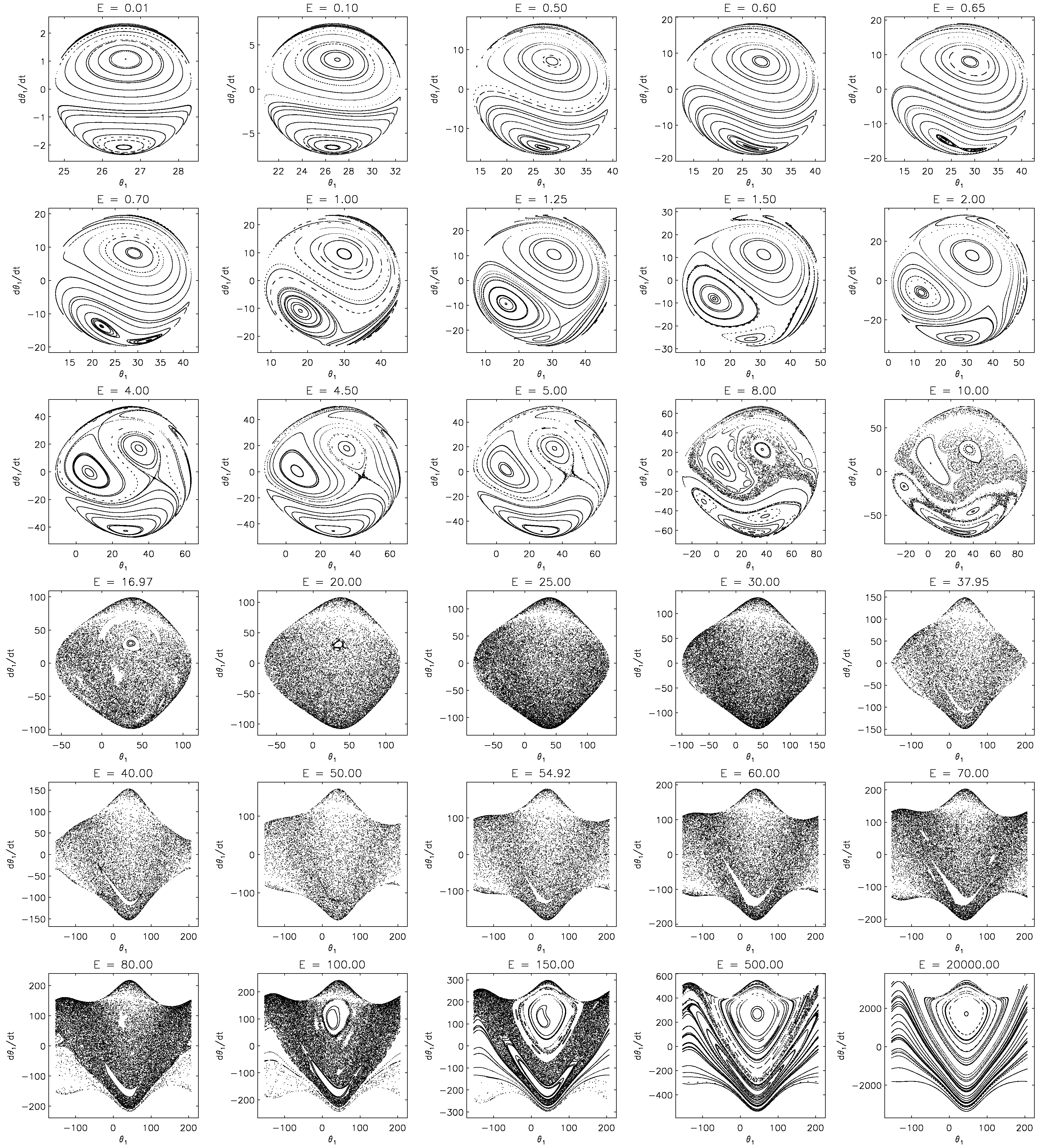
The behaviour of the pendulum varies from regular (periodic and quasi-periodic) motion at low energies, through chaos at intermediate energies, and back to regular behaviour at large energies. At large energies the pendulum acts as a rotor, with the outer plate thrown outwards. There is a simple argument that, at large energies, the motion cannot be chaotic: once the kinetic energy is large enough, the potential energy terms are negligible, and gravity is unimportant. In that case, total angular momentum is conserved, in addition to total energy. The pendulum, which has two degrees of freedom, then has two conserved quantities, and this implies that its behaviour cannot be chaotic.

The general motion at low energy is a combination of the two normal modes, and is regular.

The behaviour of the pendulum at a given energy may be summarised by a diagram called a Poincare section. For a given set of initial conditions, the equations of motion are integrated (see this page for details). Whenever the lower plate passes through its stable equilibrium position with a positive momentum, the position and speed of the upper plate is recorded, and this gives a point in the Poincare section. In terms of the animations on this page, a point in the section is produced when the cross on the outer plate passes through the vertical dotted line, from left to right, with the outer plate hanging down. The equations of motion are integrated for sufficient time to produce many points in the section. This procedure is then repeated, for different choices of initial conditions. Periodic motion of the pendulum produces a finite number of distinct points in a Poincare section (the pendulum returns to the same configuration after a certain number of equilibrium passages).

The upper figure on the right is the Poincare section for energy E = 0.01, in units of mgL/12, where m is the mass of each plate, L is the length of a side, and g is the acceleration due to gravity. The points located at about (26.6,1.06) and (26.6,-2.10) in the diagram correspond to the normal modes identified above. When the pendulum is started in one of these modes, it remains in the mode, and produces just a single point in the section. The slow mode is the upper point, and the fast mode is the lower point. Around these points are elliptical curves which correspond to quasi-periodic motion, in which the plates do not return to the same configuration in one oscillation, but return to almost the same configuration after a number of oscillations. Regular motion consists of periodic, or quasi-periodic motion. The whole diagram is approximately symmetric about a vertical line corresponding to the upper plate being at 26.6 degrees, which is the equilibrium angle for the upper plate.

The centre figure on the right shows a second Poincare section, for E = 0.65. In this case the pendulum begins to reveal its asymmetry (which is due to the centre of mass of the upper plate being offset to the right). The lower periodic point, corresponding to the fast normal mode, splits into two points, a bifurcation which has no counterpart for the simple double pendulum. However, the observed behaviour is still regular.

Irregular (chaotic) behaviour begins to appear around E = 4. Chaos appears as a scattering of points around the Poincare section, within the energetically accessible region in the section. The lower figure on the right shows the case E = 4, and points start to scatter around the X-shaped structure at (42.9,-4.65). This illustrates the onset of chaos. Initially only a limited set of initial conditions lead to irregular behaviour.

Main page on the double square pendulum
Modelling and numerical solution
Dynamics 2: Poincare sections and animations for intermediate energy
Dynamics 3: Poincare sections and animations for high energy
Images and videos of the device
Simple double pendulum page
Mike Wheatland's home page